20.4. Chokepoints Monitor - Methodology#
The Data Lab at the World Bank used IMF PortWatch to study the Red Sea shipping crisis. This event began in October 2023, when missile attacks on ships and tankers traversing the Red Sea caused hundreds of vessels to avoid the Suez Canal. The attacks are concentrated near the Bab al-Mandab Strait, a 20-mile-wide chokepoint for maritime traffic.
The following example is based on the commented study.
20.4.1. Chokepoints of interest#
The first step is to detect the chokepoints of interest. Since the example is based on the Red Sea crisis, it studies the following chokepoints:
Bab el-Mandeb Strait
Cape of Good Hope
Suez Canal
# Use already downloaded chokepoints
cpoi = ["Bab el-Mandeb Strait", "Cape of Good Hope", "Suez Canal"]
chokepoints_rs = chokepoints_gdf[chokepoints_gdf['portname'].isin(cpoi)]
chokepoints_rs
| portid | portname | country | ISO3 | continent | fullname | lat | lon | vessel_count_total | vessel_count_container | vessel_count_dry_bulk | vessel_count_general_cargo | vessel_count_RoRo | vessel_count_tanker | industry_top1 | industry_top2 | industry_top3 | share_country_maritime_import | share_country_maritime_export | LOCODE | pageid | countrynoaccents | ObjectId | geometry | |
|---|---|---|---|---|---|---|---|---|---|---|---|---|---|---|---|---|---|---|---|---|---|---|---|---|
| 0 | chokepoint1 | Suez Canal | None | None | None | Suez Canal | 30.593346 | 32.436882 | 22217 | 6455 | 5870 | 2097 | 876 | 6919 | Mineral Products | Vegetable Products | Chemical & Allied Industries | None | None | None | c57c79bf612b4372b08a9c6ea9c97ef0 | None | 1 | POINT (32.43688 30.59335) |
| 3 | chokepoint4 | Bab el-Mandeb Strait | None | None | None | Bab el-Mandeb Strait | 12.788597 | 43.349545 | 22519 | 6280 | 5940 | 1839 | 1074 | 7386 | Mineral Products | Chemical & Allied Industries | Vegetable Products | None | None | None | 6b1814d64903461b98144a6cc25eb79c | None | 4 | POINT (43.34954 12.7886) |
| 6 | chokepoint7 | Cape of Good Hope | None | None | None | Cape of Good Hope | -34.927286 | 20.882737 | 17332 | 2018 | 10277 | 709 | 355 | 3973 | Mineral Products | Vegetable Products | Prepared Foodstuffs & Beverages | None | None | None | edf18f455a2b4637a3632b6af201abe9 | None | 7 | POINT (20.88274 -34.92729) |
chokepoints_rs[
    [
        "geometry",
        "portname",
        "vessel_count_total",
        "vessel_count_container",
        "vessel_count_dry_bulk",
        "vessel_count_general_cargo",
        "vessel_count_RoRo",
        "vessel_count_tanker",
        "industry_top1",
        "industry_top2",
        "industry_top3",
    ]
].explore(
    column="portname",
    cmap="Dark2",
    marker_kwds={"radius": 15},
    tiles="Esri Ocean Basemap",
    legend_kwds={"loc": "upper right", "caption": "Choke Points"},
)
20.4.2. Retrieve the data#
The example processes the daily transit calls and estimated volume (capacity) since 2019 for the three chokepoints of interest: Bab el-Mandeb Strait, Cape of Good Hope, Suez Canal.
To build the URL for the API call, first, go to IMF PortWatch site and build a sample URL. The one below was created to retrieve information for chokepoint 1, 4, and 7. This will be useful for creating a function to retrieve the daily calls for the chokepoints of interest.
The function also needs to take into account that IMF PortWatch only returns 1000 records per call.
def get_chokepoint_data(chokepoints, url_base):
    for chokepoint in chokepoints:
        if chokepoint == chokepoints[-1]:
            url_base += f"portid%3D%20'{chokepoint}'%20&outFields=*&outSR=4326&f=json&resultOffset=0"
        else:
            url_base += f"portid%3D%20'{chokepoint}'%20+OR+"
    res = requests.get(url_base)
    df = pd.DataFrame([d["attributes"] for d in res.json()["features"]])
    offset = 1000
    while len(df) % 1000 == 0: #retrieve 1000 records
        res = requests.get(url_base.replace("resultOffset=0", f"resultOffset={offset}"))
        df2 = pd.DataFrame([d["attributes"] for d in res.json()["features"]])
        df = pd.concat([df, df2])
        offset += 1000
    df.reset_index(inplace=True, drop=True)
    df["date"] = df.date.apply(lambda x: datetime.fromtimestamp(x / 1000))
    df.sort_values(["portid", "date"], inplace=True)
    return df
url_base = "https://services9.arcgis.com/weJ1QsnbMYJlCHdG/arcgis/rest/services/Daily_Chokepoints_Data/FeatureServer/0/query?where="
df_chokepoints = get_chokepoint_data(list(chokepoints[chokepoints['portname'].isin(cpoi)].portid.unique()), url_base)
df_chokepoints.loc[:, "ymd"] = df_chokepoints.date.dt.strftime("%Y-%m-%d")
df_chokepoints.head()
| date | year | month | day | portid | portname | n_container | n_dry_bulk | n_general_cargo | n_roro | n_tanker | n_cargo | n_total | capacity_container | capacity_dry_bulk | capacity_general_cargo | capacity_roro | capacity_tanker | capacity_cargo | capacity | ObjectId | ymd | |
|---|---|---|---|---|---|---|---|---|---|---|---|---|---|---|---|---|---|---|---|---|---|---|
| 0 | 2018-12-31 21:00:00 | 2019 | 1 | 1 | chokepoint1 | Suez Canal | 23 | 22 | 14 | 4 | 22 | 63 | 85 | 1.937886e+06 | 9.439567e+05 | 174972.926920 | 46461.102534 | 1.326360e+06 | 3.103276e+06 | 4.429637e+06 | 1 | 2018-12-31 |
| 2 | 2019-01-01 21:00:00 | 2019 | 1 | 2 | chokepoint1 | Suez Canal | 26 | 4 | 6 | 5 | 10 | 41 | 51 | 2.647842e+06 | 2.389135e+05 | 33158.163236 | 99397.705404 | 6.181574e+05 | 3.019311e+06 | 3.637469e+06 | 3 | 2019-01-01 |
| 4 | 2019-01-02 21:00:00 | 2019 | 1 | 3 | chokepoint1 | Suez Canal | 12 | 16 | 10 | 3 | 24 | 41 | 65 | 7.566682e+05 | 1.050450e+06 | 81769.437679 | 50061.205601 | 1.069216e+06 | 1.938949e+06 | 3.008165e+06 | 5 | 2019-01-02 |
| 5 | 2019-01-03 21:00:00 | 2019 | 1 | 4 | chokepoint1 | Suez Canal | 18 | 13 | 1 | 1 | 15 | 33 | 48 | 1.668678e+06 | 5.830442e+05 | 1028.904676 | 16193.424839 | 1.102152e+06 | 2.268945e+06 | 3.371097e+06 | 6 | 2019-01-03 |
| 7 | 2019-01-04 21:00:00 | 2019 | 1 | 5 | chokepoint1 | Suez Canal | 20 | 9 | 1 | 1 | 13 | 31 | 44 | 1.982599e+06 | 7.714141e+05 | 1542.093497 | 16313.755096 | 6.854480e+05 | 2.771869e+06 | 3.457317e+06 | 8 | 2019-01-04 |
20.4.3. Data Smoothening#
A 7-day moving average was created to smoothen out the data and mitigate the effect of daily anomalies.
df_chokepoints = df_chokepoints.loc[df_chokepoints.date >= "2019-01-01"].copy()
df_chokepoints = (
    df_chokepoints.groupby("portname")[["n_tanker", "n_cargo", "n_total", "capacity", "date"]]
    .rolling(7, center=True, min_periods=1, on="date")
    .mean()
)
df_chokepoints.reset_index(inplace=True)
df_chokepoints.drop("level_1", axis=1, inplace=True)
df_chokepoints.loc[:, "ymd"] = df_chokepoints.date.dt.strftime("%Y-%m-%d")
df_chokepoints.loc[:, "md"] = df_chokepoints.date.dt.strftime("%m-%d")
df_chokepoints.head()
| portname | capacity | n_cargo | n_tanker | n_total | date | ymd | md | |
|---|---|---|---|---|---|---|---|---|
| 0 | Bab el-Mandeb Strait | 3.888476e+06 | 42.000000 | 18.250000 | 60.250000 | 2019-01-01 21:00:00 | 2019-01-01 | 01-01 |
| 1 | Bab el-Mandeb Strait | 3.866908e+06 | 40.600000 | 18.200000 | 58.800000 | 2019-01-02 21:00:00 | 2019-01-02 | 01-02 |
| 2 | Bab el-Mandeb Strait | 3.822667e+06 | 41.000000 | 18.166667 | 59.166667 | 2019-01-03 21:00:00 | 2019-01-03 | 01-03 |
| 3 | Bab el-Mandeb Strait | 3.693581e+06 | 40.428571 | 17.714286 | 58.142857 | 2019-01-04 21:00:00 | 2019-01-04 | 01-04 |
| 4 | Bab el-Mandeb Strait | 3.614515e+06 | 38.857143 | 17.714286 | 56.571429 | 2019-01-05 21:00:00 | 2019-01-05 | 01-05 |
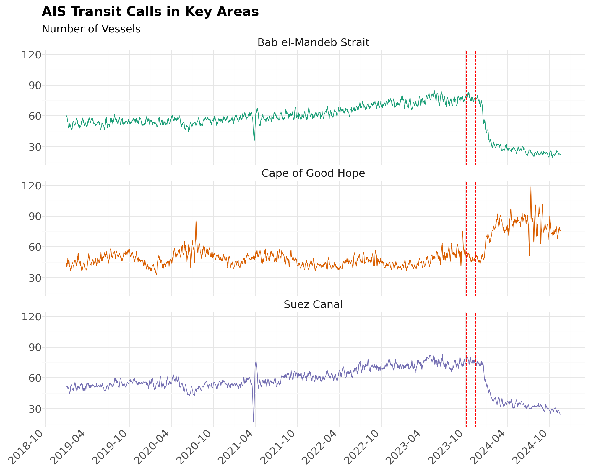
20.4.4. AIS Transit Calls in Key Areas, Historical#
This notebook uses plotnine, a package that allows to use the grammar of graphics in Python. The library is based on the famous ggplot2 library in R.
conflict_date = "2023-10-07"
crisis_date = "2023-11-17"
p0 = (
    ggplot(df_chokepoints, aes(x="date", y="n_total", group="portname", color="portname"))  #
    + geom_line(alpha=1, size=0.4)
    + geom_vline(xintercept=conflict_date, linetype="dashed", color="red")
    + geom_vline(xintercept=crisis_date, linetype="dashed", color="red")
    + labs(
        x="",
        y="",
        subtitle="Number of Vessels",
        title="AIS Transit Calls in Key Areas",
        color="Area of Interest",
    )
    + theme_minimal()
    + scale_x_datetime(breaks=date_breaks("6 month"), labels=date_format("%Y-%m"))
    + scale_color_brewer(type="qual", palette=2)
    + theme(
        text=element_text(size=13),
        plot_title=element_text(size=16, weight="bold"),
        axis_text_x=element_text(rotation=45, hjust=1),
        legend_position="none",
    )
    + facet_wrap("~portname", scales="fixed", ncol=1)
)
display(p0)
p0.save(
    filename="transit-calls-chokepoints-historical.jpeg",
    dpi=300,
)
/home/sol/venv/lib/python3.10/site-packages/plotnine/ggplot.py:606: PlotnineWarning: Saving 10 x 8 in image.
/home/sol/venv/lib/python3.10/site-packages/plotnine/ggplot.py:607: PlotnineWarning: Filename: transit-calls-chokepoints-historical.jpeg
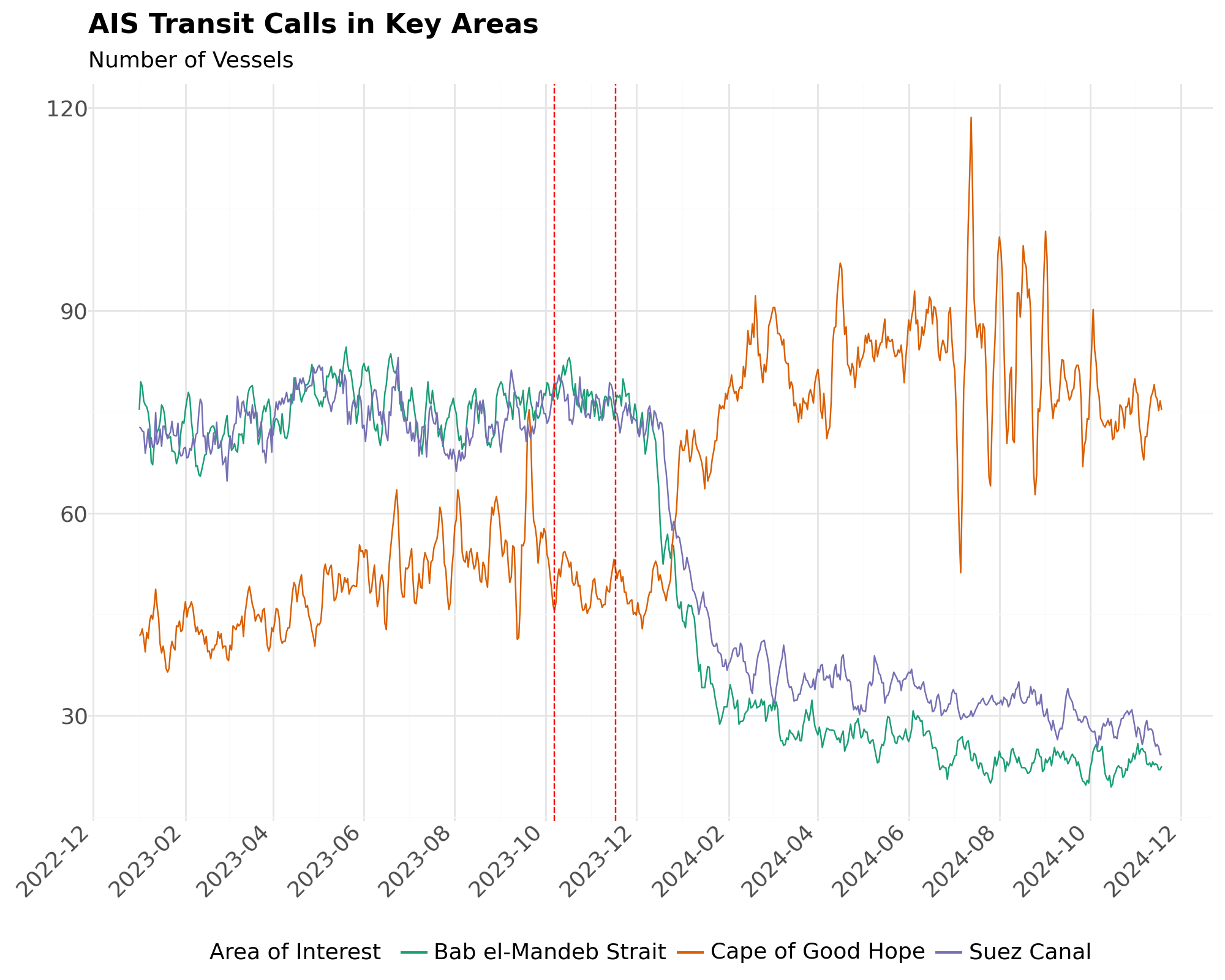
20.4.5. Reference Period#
Given the volatility of 2021, the team defined the reference period as January 1st 2022 up to October 6th 2023. Daily averages were calculated based on this time period.
Periods:
Baseline: 2021, 2022, 2023 (January 1st – October 6th)
Middle East Conflict: 2023 (October 7th - November 16th)
Red Sea Crisis: November 17th - January 31st, 2024
start_reference_date = "2022-01-01"
conflict_date = "2023-10-07"
crisis_date = "2023-11-17"
Create the reference data by day and month.
df_ref = df_chokepoints.loc[(df_chokepoints.date >= start_reference_date) & (df_chokepoints.date < conflict_date)].copy()
df_ref = df_ref.groupby(["portname", "md"])[
    ["n_tanker", "n_cargo", "n_total", "capacity"]
].mean()
df_ref.reset_index(inplace=True)
df_ref.rename(
    columns={
        "n_tanker": "n_tanker_ref",
        "n_cargo": "n_cargo_ref",
        "n_total": "n_total_ref",
        "capacity": "capacity_ref",
    },
    inplace=True,
)
Filter recent data (2023 onwards) and merge it with the reference values by day and month.
df_filt = df_chokepoints.loc[(df_chokepoints.date >= "2023-01-01")].copy()
df_filt = df_filt.merge(df_ref, on=["portname", "md"], how="left", validate="m:1")
Calculate percentage change.
df_filt.loc[:, "n_total_pct_ch"] = df_filt.apply(
    lambda x: (x.n_total - x.n_total_ref) / (x.n_total_ref), axis=1
)
p1 = (
    ggplot(df_filt, aes(x="ymd", y="n_total", group="portname", color="portname"))  #
    + geom_line(alpha=1)
    + geom_vline(xintercept=conflict_date, linetype="dashed", color="red")
    + geom_vline(xintercept=crisis_date, linetype="dashed", color="red")
    + labs(
        x="",
        y="",
        subtitle="Number of Vessels",
        title="AIS Transit Calls in Key Areas",
        color="Area of Interest",
    )
    + theme_minimal()
    + theme(
        text=element_text(size=13),
        plot_title=element_text(size=16, weight="bold"),
        axis_text_x=element_text(rotation=45, hjust=1),
        legend_position="none",
    )
    + scale_x_datetime(breaks=date_breaks("2 month"), labels=date_format("%Y-%m"))
    + scale_color_brewer(type="qual", palette=2)
    + theme(legend_position="bottom")
)
display(p1)
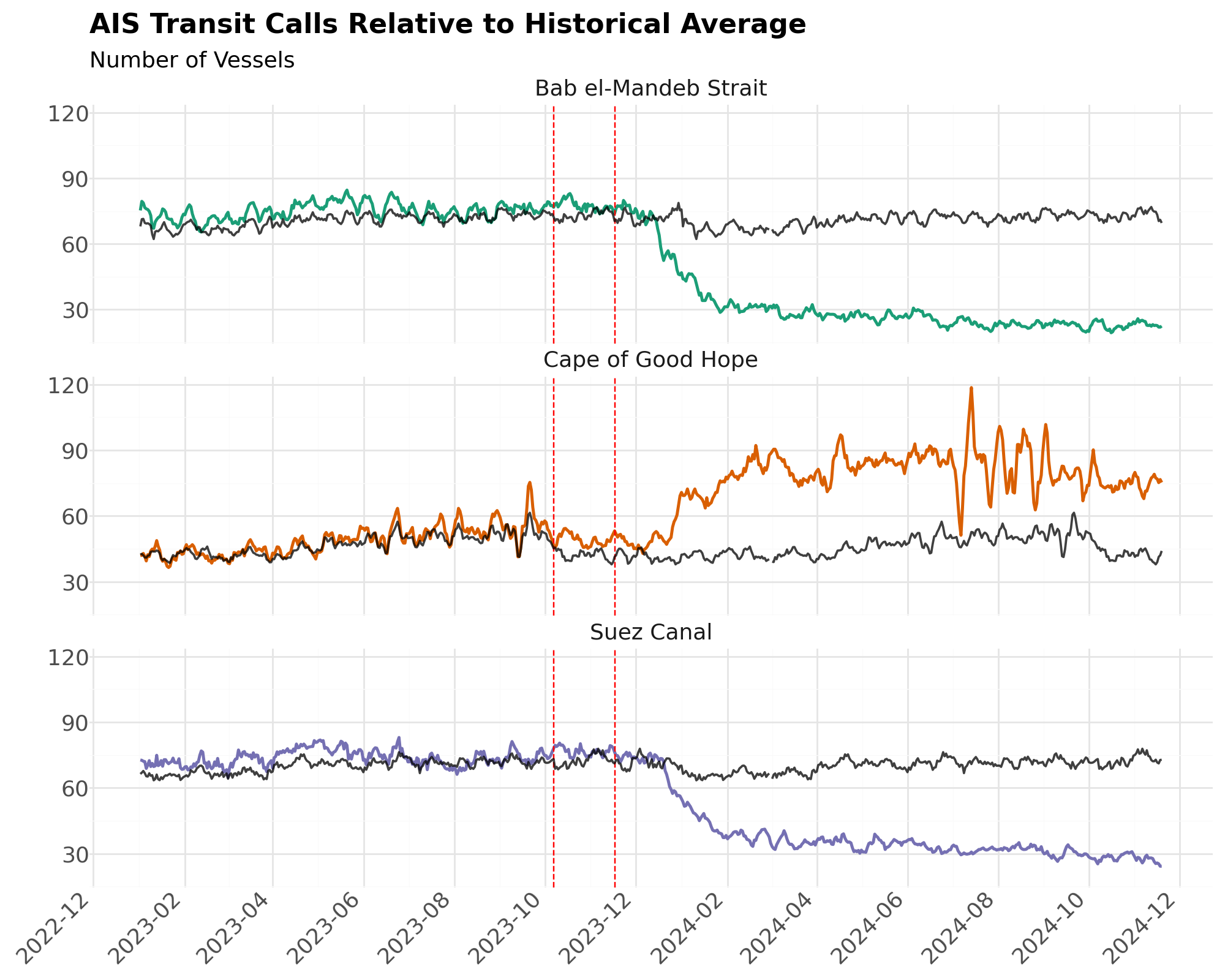
20.4.5.1. AIS Transit Calls Relative to Historical Average#
The following chart separates transit calls for each area and includes a black line, which signals the historical average for each area.
p2 = (
    ggplot(df_filt, aes(x="date", y="n_total", group="portname", color="portname"))
    + geom_line(size=1)
    + geom_vline(xintercept=conflict_date, linetype="dashed", color="red")
    + geom_vline(xintercept=crisis_date, linetype="dashed", color="red")
    + geom_line(
        aes(x="date", y="n_total_ref", group="portname"),
        color="black",
        size=0.75,
        alpha=3 / 4,
    )
    + labs(
        x="",
        y="",
        subtitle="Number of Vessels",
        title="AIS Transit Calls Relative to Historical Average",
        color="Area of Interest",
    )
    + theme_minimal()
    + theme(
        text=element_text(size=13),
        plot_title=element_text(size=16, weight="bold"),
        axis_text_x=element_text(rotation=45, hjust=1),
        legend_position="none",
    )
    + scale_x_datetime(breaks=date_breaks("2 month"), labels=date_format("%Y-%m"))
    + scale_color_brewer(type="qual", palette=2)
    + facet_wrap("~portname", scales="fixed", ncol=1)
)
display(p2)
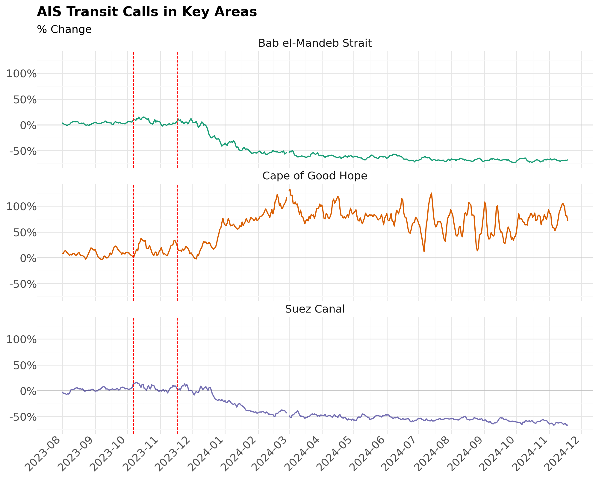
20.4.5.2. AIS Transit Calls % Change from Historical Average#
The percentage change between recent daily values and the baseline daily average was calculated.
p3 = (
    ggplot(
        df_filt.loc[df_filt.date >= "2023-08-01"],
        aes(x="ymd", y="n_total_pct_ch", group="portname", color="portname"),
    )  #
    + geom_line(size=0.8)
    + geom_vline(xintercept=conflict_date, linetype="dashed", color="red")
    + geom_vline(xintercept=crisis_date, linetype="dashed", color="red")
    + geom_hline(yintercept=0, color="black", alpha=3 / 4, size=0.3)
    + labs(
        x="",
        y="",
        subtitle="% Change",
        title="AIS Transit Calls in Key Areas",
        color="Area of Interest",
    )
    + theme_minimal()
    + theme(
        text=element_text(size=13),
        plot_title=element_text(size=16, weight="bold"),
        axis_text_x=element_text(rotation=45, hjust=1),
        legend_position="none",
    )
    + scale_x_datetime(breaks=date_breaks("1 month"), labels=date_format("%Y-%m"))
    + scale_color_brewer(type="qual", palette=2)
    + scale_y_continuous(labels=percent_format())
    + facet_wrap("~portname", scales="fixed", ncol=1)
)
display(p3)
20.4.6. Summary Statistics#
Finally, aggregate statistics (average values) per area for each period of interest were calculated.
Baseline: January 1st, 2022 – October 6th, 2023
Middle East Conflict: October 7th, 2023 - November 16th, 2023
Red Sea Crisis: November 17th, 2023 - February 19th, 2024
# Define the periods
df_chokepoints.loc[:, "period"] = ""
df_chokepoints.loc[
    (df_chokepoints.date >= start_reference_date) & (df_chokepoints.date < crisis_date), "period"
] = "Reference"
df_chokepoints.loc[
    (df_chokepoints.date >= conflict_date) & (df_chokepoints.date < crisis_date), "period"
] = "Middle East Conflict"
df_chokepoints.loc[(df_chokepoints.date >= crisis_date), "period"] = "Red Sea Crisis"
# Aggregate the data
df_agg = (
    df_chokepoints.loc[df_chokepoints.period != ""]
    .groupby(["portname", "period"])[["n_tanker", "n_cargo", "n_total", "capacity"]]
    .mean()
)

# Change order of rows
df_agg = df_agg.reindex(
    ["Reference", "Middle East Conflict", "Red Sea Crisis"], level=1
)
20.4.6.1. Table: Daily Average Values by Time Period#
table = df_agg.copy()
# Format column numbers to 2 decimal places only for first three columns
table.iloc[:, :3] = table.iloc[:, :3].apply(lambda x: round(x, 2))
# Format last column numbers to thousands
table.loc[:, "capacity"] = table.capacity.apply(lambda x: "{:,.0f}".format(x))

table.rename(
    columns={
        "n_tanker": "Tankers",
        "n_cargo": "Cargo",
        "n_total": "Total",
        "capacity": "Capacity",
    },
    inplace=True,
)
table.index.names = ["Area of Interest", "Period"]
display(table)
/tmp/ipykernel_36513/3454507845.py:5: FutureWarning: Setting an item of incompatible dtype is deprecated and will raise in a future error of pandas. Value '['4,386,509' '4,832,362' '1,551,873' '3,848,942' '4,192,709' '6,372,572'
 '4,308,488' '4,773,776' '1,881,587']' has dtype incompatible with float64, please explicitly cast to a compatible dtype first.
| Tankers | Cargo | Total | Capacity | ||
|---|---|---|---|---|---|
| Area of Interest | Period | ||||
| Bab el-Mandeb Strait | Reference | 23.96 | 46.91 | 70.87 | 4,386,509 |
| Middle East Conflict | 25.95 | 51.54 | 77.49 | 4,832,362 | |
| Red Sea Crisis | 10.67 | 20.94 | 31.62 | 1,551,873 | |
| Cape of Good Hope | Reference | 9.35 | 36.69 | 46.04 | 3,848,942 |
| Middle East Conflict | 10.03 | 39.13 | 49.15 | 4,192,709 | |
| Red Sea Crisis | 16.85 | 60.11 | 76.95 | 6,372,572 | |
| Suez Canal | Reference | 23.13 | 46.98 | 70.12 | 4,308,488 |
| Middle East Conflict | 25.20 | 51.54 | 76.74 | 4,773,776 | |
| Red Sea Crisis | 12.84 | 25.43 | 38.27 | 1,881,587 |
20.4.6.2. Table: Daily Average Values by Time Period, % Change from Baseline#
df_agg_copy = df_agg.copy()
res = []
for aoi in cpoi:
    df_sub = df_agg_copy.loc[(aoi), :].transpose().copy()
    df_sub.loc[:, "Middle East Conflict"] = (
        df_sub.loc[:, "Middle East Conflict"] - df_sub.loc[:, "Reference"]
    ) / df_sub.loc[:, "Reference"]
    df_sub.loc[:, "Red Sea Crisis"] = (
        df_sub.loc[:, "Red Sea Crisis"] - df_sub.loc[:, "Reference"]
    ) / df_sub.loc[:, "Reference"]
    df_sub2 = df_sub.transpose()
    df_sub2.drop("Reference", inplace=True)
    df_sub2.loc[:, "portname"] = aoi
    res.append(df_sub2)
df_agg_pct = pd.concat(res)
df_agg_pct.reset_index(inplace=True)
df_agg_pct.set_index(["portname", "period"], inplace=True)

# Format columns as pct
df_agg_pct = df_agg_pct.applymap(lambda x: "{:.2%}".format(x))
df_agg_pct.rename(
    columns={
        "n_tanker": "Tankers",
        "n_cargo": "Cargo",
        "n_total": "Total",
        "capacity": "Capacity",
    },
    inplace=True,
)
df_agg_pct.index.names = ["Area of Interest", "Period"]
display(df_agg_pct)
/tmp/ipykernel_36513/3184510119.py:5: FutureWarning: DataFrame.applymap has been deprecated. Use DataFrame.map instead.
| Tankers | Cargo | Total | Capacity | ||
|---|---|---|---|---|---|
| Area of Interest | Period | ||||
| Bab el-Mandeb Strait | Middle East Conflict | 8.29% | 9.86% | 9.33% | 10.16% |
| Red Sea Crisis | -55.46% | -55.36% | -55.39% | -64.62% | |
| Cape of Good Hope | Middle East Conflict | 7.22% | 6.65% | 6.77% | 8.93% |
| Red Sea Crisis | 80.14% | 63.84% | 67.15% | 65.57% | |
| Suez Canal | Middle East Conflict | 8.92% | 9.70% | 9.45% | 10.80% |
| Red Sea Crisis | -44.50% | -45.87% | -45.42% | -56.33% |