18. Night Time Lights to estimate Disruptions to Business and Trade

18.1. Summary

In our previous class about NTL we studied how to use Black Marble’s dataset to understand how crises affected their surrounding areas. You learned to plot weekly and monthly radiance time series and a time series showing percentage change in radiance with respect to a baseline before the crisis event. These indicators allowed us to understand population movements as a consequence of a crisis event. In this class, we want to use NTL data to understand the disruptions a crisis can generate to business and trade. We will be calculating the change in NTL for areas with and without gas flaring and the correlation between NTL and GDP. The class focuses on the methodology employed by the Data Lab for the Myanmar Economic Monitor.

18.2. Learning Objectives

18.2.1. Overall goals

The main goal of this class is to teach students to leverage NTL data for assessing the economical impact of a crisis.

18.2.2. Specific goals

At the end of this notebook, you should have gained an understanding and appreciation of the following:

1. Use NTL as a proxy of economical activity:

   • What data can be used in tandem with NTL for assessing economical impact.

   • Combine NTL with GDP.

   • Understand the limitations of this dataset.

18.3. Download the data

The area of interest can be downlaod from GADM, with administrative levels from 0 to 3.

The data is downloaded using BlackMarblePy. The downloaded products are VNP46A4 and VNP46A3, which will be aggregated at different levels. Since the project uses different aggregation levels for each product, we will download the output files locally to avoid redownloading them each time a different aggregation is performed.

import os
import pandas as pd
import geopandas as gpd
from shapely import Point
from datetime import datetime
import requests
from scipy.stats import pearsonr

from blackmarble.extract import bm_extract
from blackmarble.raster import bm_raster, transform

from plotnine import *
from mizani.breaks import date_breaks
from mizani.formatters import date_format, percent_format, comma_format, scientific_format
import matplotlib.pyplot as plt

admin0 = gpd.read_file('../../data/ntl-disruptions-business/gadm41_MMR.gpkg', layer = 'ADM_ADM_0')
admin1 = gpd.read_file('../../data/ntl-disruptions-business/gadm41_MMR.gpkg', layer = 'ADM_ADM_1')
admin2 = gpd.read_file('../../data/ntl-disruptions-business/gadm41_MMR.gpkg', layer = 'ADM_ADM_2')

bearer = os.getenv('bm_token')

VNP46A4_admin0 = bm_extract(
                            admin0,
                            product_id="VNP46A4",
                            date_range=pd.date_range("{}-01-01".format(2012), "{}-12-31".format(2024), freq="MS"),
                            bearer=bearer,
                            aggfunc=["mean", "sum"],
                            output_directory="./ntl/",
                            output_skip_if_exists=True                            
                        )

VNP46A4_admin1 = bm_extract(
                            admin1,
                            product_id="VNP46A4",
                            date_range=pd.date_range("{}-01-01".format(2012), "{}-12-31".format(2024), freq="MS"),
                            bearer=bearer,
                            aggfunc=["mean", "sum"],
                            output_directory="./ntl/",
                            output_skip_if_exists=True                            
                        )

VNP46A4_admin2 = bm_extract(
                            admin2,
                            product_id="VNP46A4",
                            date_range=pd.date_range("{}-01-01".format(2019), "{}-12-31".format(2024), freq="MS"),
                            bearer=bearer,
                            aggfunc=["mean", "sum"],
                            output_directory="./ntl/",
                            output_skip_if_exists=True                            
                        )

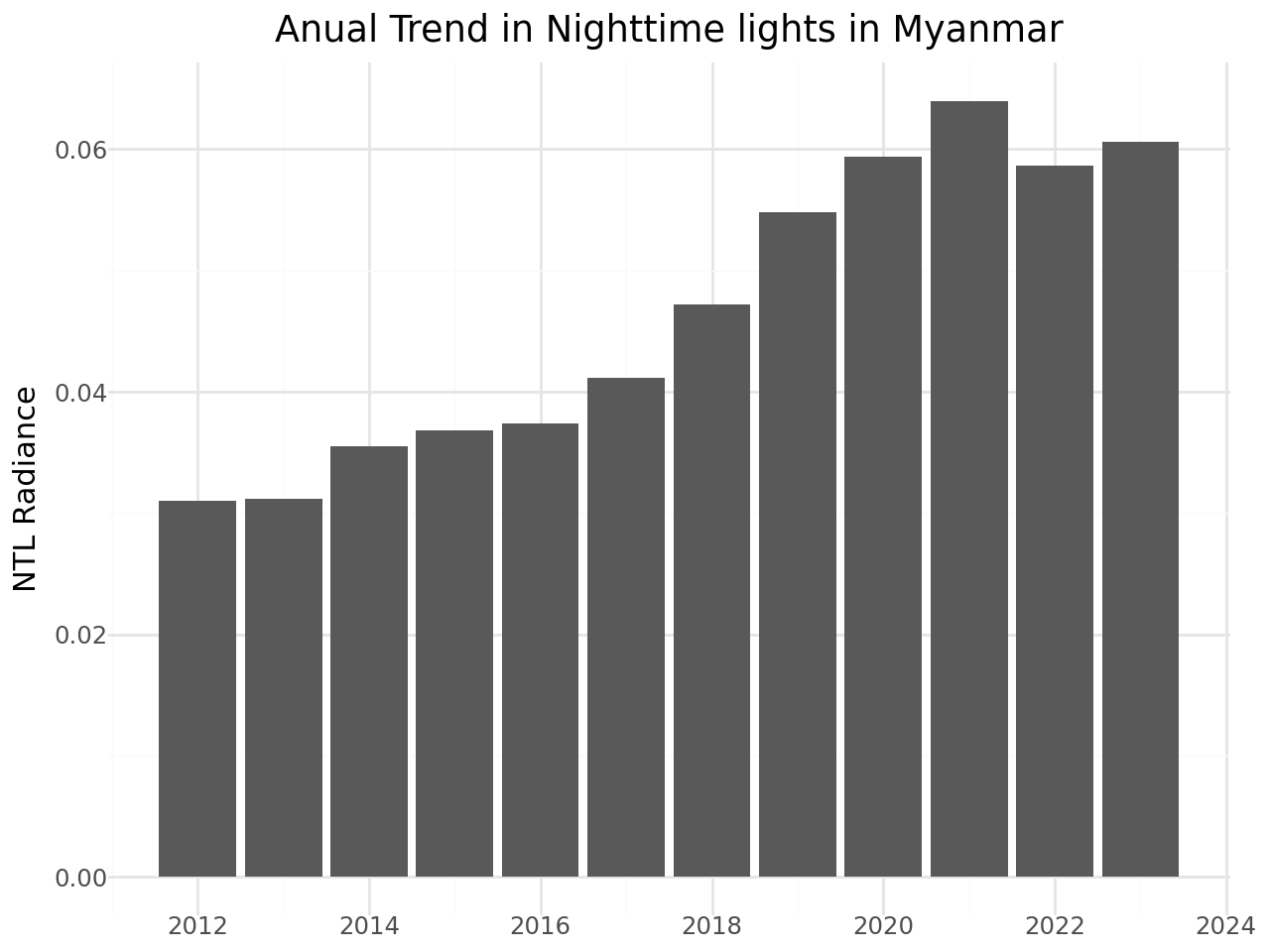
18.4. Annual Trends in Nighttime Lights - Country level

annual_trend_admin0 = (
    ggplot(VNP46A4_admin0, aes(x = 'date', y = 'ntl_mean'))
    + geom_col()
    + labs(x = "",
       y = "NTL Radiance",
       title = "Anual Trend in Nighttime lights in Myanmar")
    + theme_minimal()
    + scale_x_datetime(breaks=date_breaks("2 year"), labels=date_format("%Y"))
    )
display(annual_trend_admin0)

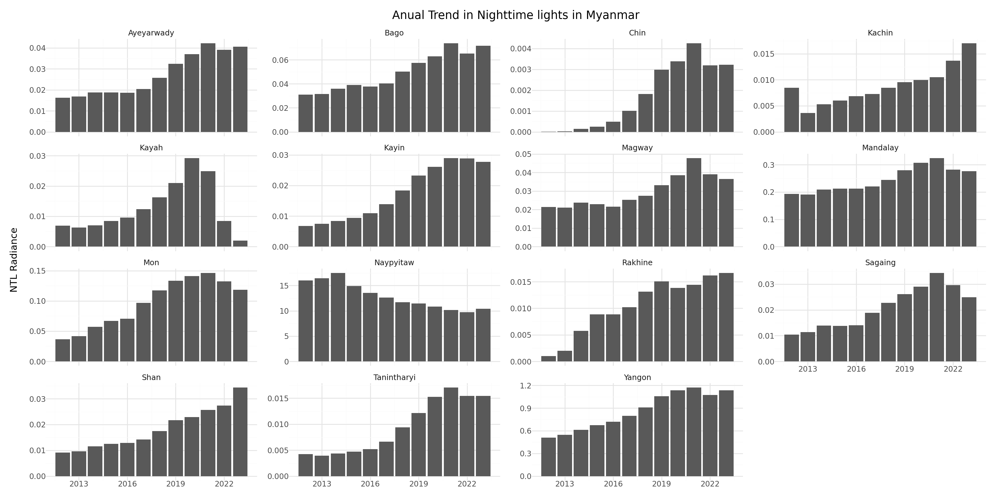
18.5. Annual Trends in Nighttime Lights - Administrative level 1

annual_trend_admin1 = (
    ggplot(VNP46A4_admin1, aes(x = 'date', y = 'ntl_mean'))
    + geom_col()
    + labs(x = "",
       y = "NTL Radiance",
       title = "Anual Trend in Nighttime lights in Myanmar")
    + facet_wrap('~NAME_1', scales='free_y')
    + theme_minimal()
    + theme(figure_size=(16, 8))
    + scale_x_datetime(breaks=date_breaks("3 year"), labels=date_format("%Y"))
    )

display(annual_trend_admin1)

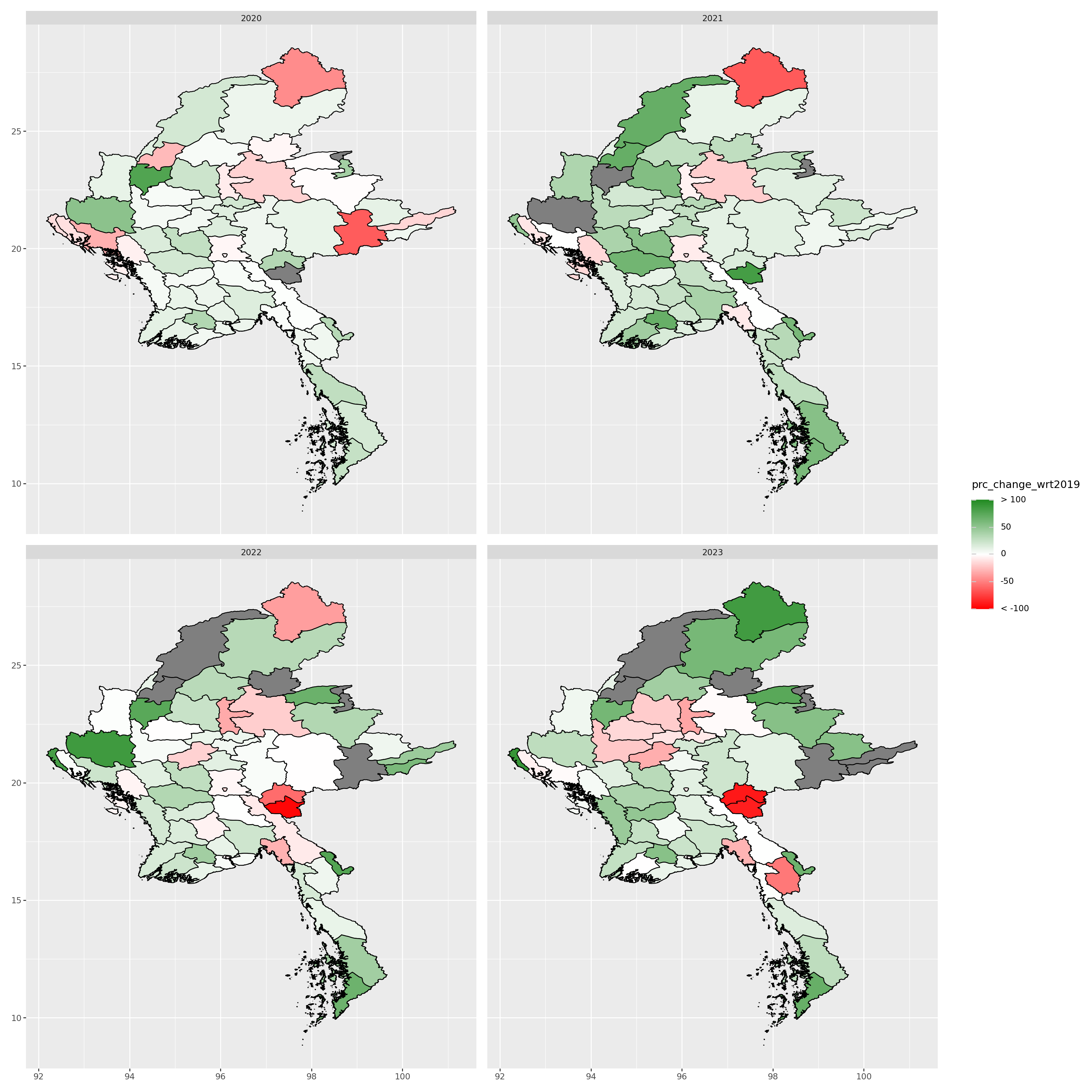
18.6. Percentage Change in NTL at Administrative Level 3 - Maps

var = 'ntl_mean'
baseline_2019 = VNP46A4_admin2[VNP46A4_admin2['date']<'2020'].groupby(['NAME_2', 'date'])[[var]].mean().reset_index(level = 1)
data = VNP46A4_admin2[VNP46A4_admin2['date']>='2020'].groupby(['NAME_2', 'date'])[[var]].mean().reset_index(level = 1)

merge = pd.merge(data, baseline_2019, left_index = True, right_index = True, suffixes=('', '_2019'), how = 'left')

merge['prc_change_wrt2019'] = merge.apply(lambda row: 100*((row[var]-row['{}_2019'.format(var)])/row['{}_2019'.format(var)]), axis = 1)
merge['year'] = merge['date'].dt.strftime("%Y")

merge = merge.merge(admin2[['NAME_2', 'geometry']], on = 'NAME_2', how = 'left')

merge_gdf = gpd.GeoDataFrame(merge, crs='EPSG:4326', geometry = merge['geometry'])

annual_trend_admin2 = (
        ggplot() 
        + geom_map(merge_gdf, aes(fill='prc_change_wrt2019'), color = 'black') 
        + facet_wrap('~year') 
    # + theme_void() 
    # + theme(plot.title = element_text(face = "bold", hjust = 0.5))
    
    # + labs(title = paste0("Percent Change in Nighttime Lights from 2019: ADM ", roi, " level"),
    #      fill = "% Change") 
    + scale_fill_gradient2(low = "red",
                         mid = "white",
                         high = "forestgreen",
                         midpoint = 0,
                         limits = [-100, 100],
                         breaks = [-100, -50, 0, 50, 100],
                         labels = ["< -100", "-50", "0", "50", "> 100"])
    + theme(figure_size=(16, 16))
)
display(annual_trend_admin2)

18.7. Gas Flaring Nighttime Lights

It is important to distinguish between lights observed in gas flaring locations and lights in other locations. Oil extraction and production involve gas flaring, which produces significant volumes of light. Separately examining lights in gas flaring and other locations allows distinguishing between lights generated due to oil production versus other sources of human activity. Data related to gas flaring sites comes from the Global Gas Flaring Reduction Partnership.

18.7.1. Gas Flaring Data

The data can be downloaded from here. Then, we spatially intersect this.

gas_flaring = pd.read_excel('../../data/ntl-disruptions-business/2012-2023-individual-flare-volume-estimates.xlsx')

def create_gdf(data, epsg, lat, lon):
    '''Create a GDF from a csv with lat and lon'''
    geometry = data.apply(lambda row: Point(row[lon], row[lat]), axis = 1)
    return gpd.GeoDataFrame(data, crs = epsg, geometry = geometry)

gas_flaring_gdf = create_gdf(gas_flaring, 'epsg:4326', 'Latitude', 'Longitude')

gas_flaring_gdf[gas_flaring_gdf['Year']==2012].explore()

Make this Notebook Trusted to load map: File -> Trust Notebook

I do not find the gas flaring locations for Myanmar

  Cell In[47], line 1
    I do not find the gas flaring locations for Myanmar
      ^
SyntaxError: invalid syntax

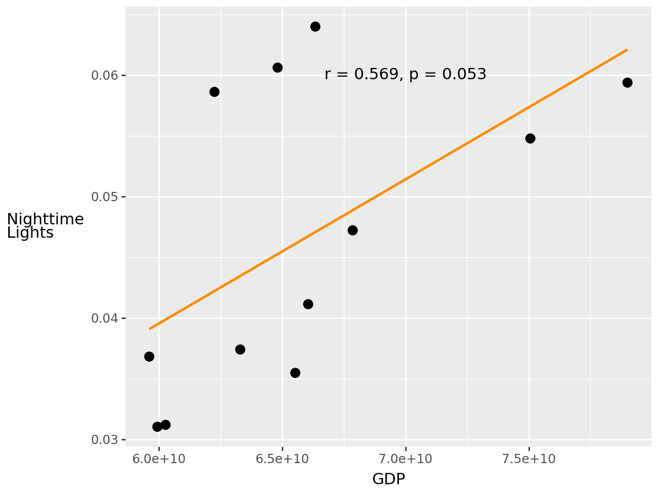
18.8. GDP vs NTL annual

This part of the analysis explores the relationship between Nighttime Lights and GDP.

gdp = pd.read_csv('../../data/ntl-disruptions-business/API_NY.GDP.MKTP.CD_DS2_en_csv_v2_2404859.csv', skiprows = 4)

# Extract data for MMR from 2012 (year in which we have Black Marble data)
gdp_mmr = gdp[gdp['Country Code']=='MMR'].copy()[[str(year) for year in range(2012, 2024)]].unstack().reset_index()
gdp_mmr.drop('level_1', axis = 1, inplace = True)
gdp_mmr.rename(columns = {'level_0': 'year', 0: 'GDP'}, inplace = True)
gdp_mmr['year'] = gdp_mmr['year'].astype('int')
gdp_mmr.set_index('year', inplace = True)

VNP46A4_admin0['year'] = VNP46A4_admin0['date'].dt.year

gdp_mmr['ntl_sum'] = VNP46A4_admin0.set_index('year')['ntl_sum']
gdp_mmr['ntl_mean'] = VNP46A4_admin0.set_index('year')['ntl_mean']

r_value, p_value = pearsonr(gdp_mmr['GDP'], gdp_mmr['ntl_mean'])

annual_gdp = (
    ggplot(gdp_mmr, aes(x = 'GDP', y = 'ntl_mean'))
    + geom_smooth(method='lm', formula='y ~ x', se=False, color="darkorange")
    + geom_point(size = 3)
    + annotate('text', x=70000000000, y=0.06, label=f'r = {round(r_value, 3)}, p = {round(p_value, 3)}', color='black')
    + labs(x = "GDP", y = "Nighttime\nLights")
    + theme(axis_title_y=element_text(angle=0, va='center'))
    + scale_x_continuous(labels=scientific_format())
    
) 
display(annual_gdp)

18.9. Limitations

Nighttime lights are a common data source for measuring local economic activity. However, it is a proxy that is strongly—although imperfectly—correlated with measures of interest, such as population, local GDP, and wealth. Consequently, care must be taken in interpreting reasons for changes in lights.