2. Modelflow methods reference

The main text of this document presents a large range of ModelFlow features in the context of where they may be used. This chapter reproduces much of that information but out of context. It is not a full technical reference to ModelFlow but it does attempt to put into place a handy reference to many of the commands that a ModelFlow user of the World Bank models would need. Ib Hansen maintains a ModelFlow reference here.

In this chapter - ModelFlow Methods Reference

This chapter provides a summary reference of the main methods of ModelFlow package. It is not comprehensive, but is meant to be used as a handy guide to the syntax of the many methods in ModelFlow. More detailed explanations of many of the methods occur in the text and can be found by consulting the index.

Features included in the reference include:

• Jupyter Notebook Integration:

  • Utilize Jupyter-specific commands and features for an interactive modeling experience.

  • Enable extensions to enhance productivity (e.g., auto-completion, variable inspection).

• Core Model Methods:

  • Manage model properties and equations with methods for adding, modifying, or deleting equations.

  • Use .dekomp() for decomposition and .tracepre() for dependency analysis.

  • Perform simulations and save results with explicit methods like .solve() and .pcim.

• DataFrame Manipulations:

  • Leverage ModelFlow extensions to pandas for time-series analysis and variable transformations.

  • Use .upd() and .mfcalc() for data updates and calculated transformations.

• Visualization and Reporting:

  • Create charts and plots with .plot() and .draw() for clear data representation.

  • Build structured reports using .rtable() and .rplot() methods.

• Advanced Features:

  • Define time frames and scenarios for focused simulations.

  • Save and compare results across multiple runs for robust analysis.

In order to manipulate plots later on matplotlib.pyplot is also imported.

import matplotlib.pyplot as plt # To manipulate plots 

2.1. Useful Jupyter Notebook commands and features

2.1.1. .widescreen()

Instructs ModelFlowto take full advantage of the space available on the browser under which Jupyter Notebook is running.

model.widescreen() 

2.1.2. .scroll_off()

Instructs ModelFlow not to scroll outputs within a cell, but to show the whole output. Useful when displaying multiple charts and tables.

model.scroll_off()

latex=True #used to ensure  that outputs render well in pdf format

2.2. Working with the Model Object

The model object is the central object in ModelFLow. It’s methods are used to read and write models from disk, and to perform simulations, and to report the results of simulations both as graphs and tables. Its properties include the data associated with the model, the current options that impact simulations, the individual equations that together comprise the system of equations that the model object solves.

2.3. Selected model properties

Models once built can be saved to disk for later reloading. The entire model state can be saved, including options for the solve operator, and the results from solutions that were earlier run with the keep option.

The model state has many properties. Including:

Content	Property	Description
Model equations	.equation	Returns a very long string containing all of the equations of the model.
Model name	.name	Returns the internal name of the model. For WBG models this is typically the 3 letter ISO code for the country , i.e. PAK for Pakistan
Model description	.model_description	If defined, returns a string with a longer description of the model – otherwise returns a blank string.
Base solution	.basedf	Returns a DataFrame of all the variables in the model with the values from the baseline or initialization values of the model.
Last solution	.lastdf	Returns a DataFrame of all the variables in the model with the values from the most recently executed simulation.
Kept solutions	.keep_solutions	A dictionary of DataFrames. The key to the dictionary is the text passed to the keep=copmmand when the solution was run, and the value is the DataFrame generated by the simulation.
Current time frame	.current_per	Returns the active sample period of the model (the time-slice over which the model will be solved).
Simulation options	.oldkwargs	Returns a dictionary, showing the current state of the persistent options of the model.
Variable descriptions	.var_description	Returns a dictionary, with long form descriptions of those mnemonics in the model that have been assigned a long-form description.
User defined lists of variables	.var_groups	Returns a dictionary, showing the various groups (lists of variables) that have been defined for this model object.
Reports	.reports	Returns a Dictionary of all Reports (if any) that have been defined for the model.

2.4. Selected Model methods

2.4.1. .model_load() method: Loading models

The model_load()method instantiates (creates) a new model object from a previously saved pcim file.

Parameters:

Parameter	Type	Description
infile	string	The name of the file or URL from which the model will be loaded.
funks	list	Functions to use in the resulting model. Default is an empty list.
run	bool	If True, simulates the model with the saved time and options. Default is False.
keep_json	bool	If True, saves a dictionary (self.json_keep) in the model instance. Default is False.
default_url	string	The default URL where to look for the model if it is not in the specified location. Default value is: ‘https://raw.githubusercontent.com/IbHansen/ModelFlow-manual/main/model_repo/’,**kwargs)’
**kwargs	dict	Additional keyword arguments used by the simulation if run=True.

Returns

• tuple: A tuple containing a model instance and a DataFrame.

2.4.1.1. Load an example model and create a model instance

Also the model is run

mpak,baseline = model.modelload('../models/pak.pcim', \
         run=True,keep= 'Baseline')

Zipped file read:  ..\models\pak.pcim

The above example declares an instance of a model object mpak and a DataFrame – baseline– that holds the results of the simulation invoked by the run=True option. The keep='Baseline' instructs the method to also store the result of the initial simulation as a scenario identified by the text ‘Baseline’.

2.4.2. .model_dump() method: Saving models

The .modeldump() method saves the content of a model object to disk. By default, models are stored using the json format. By convention dumped ModelFlow objects are saved to a file with the .pcim extension.

Parameters:

Parameter	Type	Description
outfile	string	The name of the file where the model will be dumped. Default is an empty string, meaning the dump will be returned as a string.
keep	bool	If True, the keep_solutions attribute of the model will also be dumped. Default is False.

Returns

• string: If outfile is an empty string or not specified, the method returns the model dump as a JSON string.

2.4.2.1. example

mpak.modeldump('Mymodel/Mymodel',keep=True)

Saves the model object mpak to a file called Mymodel.pcim located in the Mymodel sub-directory. The model would also contain the results DataFrames for all the simulations that were stored with the keep option.

!dir Mymodel\*.pcim

 Volume in drive C is OSDisk
 Volume Serial Number is 9846-30C3

 Directory of C:\mflow\papers\mfbook\content\07_MoreFeatures\Mymodel

10/02/2025  10:34 AM         2,084,793 Mymodel.pcim
               1 File(s)      2,084,793 bytes
               0 Dir(s)  711,908,560,896 bytes free

2.5. Equations

The model object includes both the data of the model and the equations that define the relationship between the variables.

2.5.1. Fixable equations

A behavioral equation determines the value of an endogenous variable, based on an econometric relationship rather than an accounting identity. They are comprised of right-hand side variables (the regressors in the econometric relationship or the explanatory variables), left hand side variables (the regressands or dependent variable), estimated parameters, perhaps some imposed parameters, and the error term.

In addition to these elements, a fixable equation will have three special variables defined, which allow the equation to be de-activated (exogenized). These variables carry the same root mnemonmic as the equation’s dependent variable and the terminators, \(\_A\), \(\_X\), \(\_D\).

Terminator	Meaning	Role
_A	Add factor:	special variable to allow judgment to be added to an equation
_X	Exogenized value:	Special variable that stores the value that the equation should return if exogenized
_D	Exogenous dummy:	Dummy variable. When set to one, the equation will return the value of the _𝑋 variable, if zero, it returns the fitted value of the equation plus the Add factor

A standard econometric equation such as \( y_t = \hat{\alpha} + \hat{\beta} X_t + y\_A_t\) can be rewritten as

\[\begin{equation*} y_t = (1-y\_D_t)\cdot\underbrace{\biggl[\hat{\alpha} + \hat{\beta} X_t + y\_A_t\biggr]}_{\begin{array}{c} \text{Econometric equation}\end{array}} + y\_D_t\cdot \underbrace{y\_X_t}_{\begin{array}{c} \text{Exogenized} \\ \text{value} \end{array}} \end{equation*}\]

When \(y\_D_t=1\) then the first expression (the econometric equation) solves to zero and the equation just returns the value \(y\_X_t\).

2.5.2. .var_with_frmlname(‘DAMP’), Dampable variables

Returns a set of variable names of equations that can be Dampened (dampening adjusts the size of changes to a variable that are imposed when the model is trying to solve.

Below the set is made to a sorted list and the first 3 variable names are printed.

2.5.3. .wb_behavioral property: returns a list of fixable (behavioral) equations

.wb_behavioral is a property of a model object, which defines all of the behavioral (fixable) equations in the model object.

2.5.3.1. example

themodel.wb_behavioral will return a list of all the variables with fixable equations.

2.5.4. .fix() method: exogenizes one or more equations in the model.

The fix()method sets the \(\_D\) variable to 1 and the \(\_X\) variable to the value that the user wants the equation to resolve to when exogenized.

Parameters:

Parameter	Type	Description
df	TYPE	Input dataframe should contain a solution and all variables.
pat	TYPE, optional	Select variables to exogenize. Defaults to ‘*’ (All variables).
start	TYPE, optional	Start period. Defaults to ‘’.
end	TYPE, optional	End period. Defaults to ‘’.
silent	int, optional	If set to 1, suppresses print output. Defaults to 0.

Returns:

• A DataFrame.

2.5.4.1. example 1

Cfixed=themodel.fix(baseline,’PAKNECONPRVTKN’)

Returns a new DataFrame Cfixed exactly equal to the baseline DataFrame but with the PAKNECONPRVTKN_D variable set to 1. This equation will now return PAKNECONPRVTKN_X for all periods where PAKNECONPRVTKN_D is equal to 1. PAKNECONPRVTKN_X will be set equal to the current value of PAKNECONPRVTKN. To do a meaningful simulation the value of PAKNECONPRVTKN_X would have to be changed, say as below.

Cfixed=Cfixed.upd("<2025 2040> PAKNECONPRVTKN_X * 1.025") which would increase the value of consumption by 2.5% between the years 2025 and 2040.

2.5.4.2. example 2

Cfixed2=themodel.fix(baseline,’PAKNECONPRVTKN’,start=2045,end=2050)

Returns a new DataFrame Cfixed2 exactly equal to the baseline DataFrame but with the PAKNECONPRVTKN_D variable set to 1 for the years 2045 through 2050. This equation will now return PAKNECONPRVTKN_X for this period.

Cfixed=Cfixed.upd("<2025 2050> PAKNECONPRVTKN_X * 1.025") would increase the value of consumption by 2.5% for the period 2020 through 2045.

In this example the changes to PAKNECONPRVTKN_X before 2045 would have no effect as the variable was only exogenized in the preceding fix statement for the period 2045 through 2050.

2.5.5. .unfix() method:re-activates an exogenized equation

Parameters:

Parameter	Type	Description
df	Dataframe	Input dataframe, should contain a solution and all variables.
pat	string, optional	Select variables to endogenize. Defaults to ‘*’.
start	TYPE, optional	Start period. Defaults to ‘’.
end	TYPE, optional	End period. Defaults to ‘’.

Returns:

A dataframe with the _D version of the specified variables set to zero for the specified time period.

2.5.5.1. example1

Unfixed=themodel.fix(Cfixed2,'PAKNECONPRVTKN')

Creates a new DataqFrame that is a copy of Cfixed2 but with PAKNECONPRVTKN_D equal to zero over the entire period.

2.5.5.2. example2

Unfixed2=themodel.fix(Cfixed2,'PAKNECONPRVTKN','2040','2050)

Creates a new DataFrame’, unfixed2 that is a copy of Cfixed2 but with PAKNECONPRVTKN_D equal to zero over the period period 2040 through 2050. If PAKENCONPRVTKN had been exogenized for a longer period, it would remain exogenized in the periods outside of 2050- 2050.

2.5.6. .fix_inf property: Returns a list of the variables currently exogenized (fixed)

.wb_inf is a property of a model object, which returns a list of the behavioral (fixable) equations in the model object that are currently fixed (exogenized).

2.6. Visualize equations

ModelFlow offers three ways to visualize an equation.

Methods	Returns
.eviews()	returns the original EViews form of the equation (only available for models imported from EViews)
.frml()	returns the internal normalized version of the EViews equation
.show()	returns the internal normalized version of the EViews equation and data for theLHS and RHs variables of the equation from both the .basedf, .lastdf DataFrames and their differences

2.6.1. .eviews() method: Diplays the original format of the equation

mpak.PAKBXGSRMRCHCD.eviews;

DLOG(PAKBXGSRMRCHCD) = 2.82268702067837e-08*(LOG(PAKBXGSRMRCHCD( - 1)) - 505277.224656802*LOG(PAKXMKT( - 1)) - 2.91054176583784*LOG(PAKREER( - 1))) + 0.0683002735007435 + 0.167350489665585*DLOG(PAKXMKT) + 0.0611655503957304*DLOG(PAKREER)

2.6.2. .eviews() method: Displays the normalized form of the equation

mpak.PAKBXGSRMRCHCD.frml;

Endogeneous: PAKBXGSRMRCHCD: Exp., MRCH (BOP), US$ mn
Formular: FRML <DAMP,STOC> PAKBXGSRMRCHCD = (PAKBXGSRMRCHCD(-1)*EXP(PAKBXGSRMRCHCD_A+ (2.82268702067837E-08*(LOG(PAKBXGSRMRCHCD(-1))-505277.224656802*LOG(PAKXMKT(-1))-2.91054176583784*LOG(PAKREER(-1)))+0.0683002735007435+0.167350489665585*((LOG(PAKXMKT))-(LOG(PAKXMKT(-1))))+0.0611655503957304*((LOG(PAKREER))-(LOG(PAKREER(-1))))) )) * (1-PAKBXGSRMRCHCD_D)+ PAKBXGSRMRCHCD_X*PAKBXGSRMRCHCD_D  $

PAKBXGSRMRCHCD  : Exp., MRCH (BOP), US$ mn
PAKBXGSRMRCHCD_A: Add factor:Exp., MRCH (BOP), US$ mn
PAKBXGSRMRCHCD_D: Fix dummy:Exp., MRCH (BOP), US$ mn
PAKBXGSRMRCHCD_X: Fix value:Exp., MRCH (BOP), US$ mn
PAKREER         : Real Exchange Rate (Trade Weighted)
PAKXMKT         : Weighted Trading Partner Demand

2.6.3. .show() method: Displays the normalized form of the equation plus data from the .lastdf, .basedf DataFrames and their difference

with mpak.set_smpl(2024,2032):
    mpak.PAKBXGSRMRCHCD.show; 

2.7. Adding, Modifying, or Deleting Equations

Sometime it can be useful to change a model. You might need to:

• Add new equations to incorporate additional functionality or dynamics.

• Modify existing equations to refine or adjust the model’s behavior.

• Delete unnecessary equations to simplify the model or remove obsolete components.

These actions enable you to tailor the model to better meet your specific requirements.

2.7.1. .eqdelete Delete equations

Parameter	Type	Description
deleteeq	TYPE, optional	Variables where equations are to be deleted. Defaults to None.
newname	string, optional	The name of the new model with deleted equations. Defaults to an empty string.

Returns:

• newmodel: TYPE - The new model with the deleted equations.

• newdf: TYPE - A dataframe with calculated add factors. Origin is the original model’s lastdf.

2.7.2. .equpdate Update or add equations

Parameter	Type	Description
updateeq	TYPE	New equations separated by newline.
add_add_factor	bool, optional	Whether to add an add factor. Defaults to False.
calc_add	bool, optional	Whether to calculate add factors. Defaults to True.
do_preprocess	bool, optional	Whether to preprocess the equations. Defaults to True.
newname	string, optional	The name of the updated model. Defaults to an empty string.
silent	bool, optional	Whether to suppress print outputs. Defaults to True.

Returns:

• newmodel: TYPE - The updated model with new and deleted equations.

• newdf: TYPE - A dataframe with calculated add factors. Origin is the original model’s lastdf.

dampable_variables = sorted(mpak.var_with_frmlname('DAMP'))
print(f'Number of dampable variables: {len(dampable_variables)}')
print(f'First 3 dampable variables  : {dampable_variables[:3]}')

Number of dampable variables: 75
First 3 dampable variables  : ['PAKBMFSTOTHRCD', 'PAKBMFSTREMTCD', 'PAKBMGSRGNFSCD']

2.8. Manipulating DataFrames

Pandas dataframes can be extended with new functionality. When the import modelclass statement is executed ModelFlow will extend dataframes with two new capabilities.

• .upd which allows easy updating of variables (columns) in dataframes. The purpose is to facilitate relevant update operations.

• .mfcalc which enables transformations using lags and straight expressions.

2.8.1. .loc() method

2.8.2. .upd Updates a dataframe and returns a dataframe

Parameters:

Parameter	Type	Description	Default
basis	string	Lines with variable updates (see below for format).
lprint	bool, optional	If True, each update is printed.	False
scale	float, optional	A multiplier used on all update input.	1.0
create	bool, optional	Creates variables if not in the dataframe.	True
keep_growth	bool, optional	Keep the growth rate after the update time frame.	False

A line in updates looks like this:

[<[[start] end]>] <var> <=|+|*|%|=growth|+growth|=diff> <value>... [--keep_growth_rate|--kg|--no_keep_growth_rate|--nkg]

The number of values should either be one - which then is applied to all years, or the number of years from start to end.

Time carries over from line to line.

The basisstring can contain several updates separated by new line.

Returns: A new dataframe containing the updated values of the input dataframe

2.8.3. .mfcalc Updates a dataframe and returns a dataframe

This implement the model class on top of pandas dataframes. Useful to do transformations with lags.

Parameter	Type	Description	Default
eq	str	Equations, one on each line. Can be started with <start end> to control calculation sample.
start	optional	DESCRIPTION.	''
end	optional	DESCRIPTION.	''
showeq	bool, optional	If True, the equations will be printed.	False
**kwargs	optional	Here all solve options can be provided.

Each equation \(f_i\) is specified as:

<left hand side> = <right hand side> $

Each formula ends with a $.

The <left hand side> should not contain transformations. Lags or leads can not be specified at the left hand side of \(=\).

Time \(t\) is implicit in the equations which means that a \(var\) at time \(t\) written as var, while \(var_{t-1}\) is written as var(-1). ModelFlow is case-insensitive. Everything is eventually transformed into upper case.

The <right hand side> can contain variables, operators, functions

2.9. Performing Simulations

ModelFlowis a package to solve complex systems of equations. It supports a range of solution engines, each of which has different features.

2.9.1. <model instance>() method, solve the model

The most convenient way to solve a model is to call it by passing simulation parameters directly to the model instance[1].

Parameter	Type	Description
do_calc_add_factor	bool	Determines whether to calculate the add factors. Used to calculate add-factors to ensure the model exactly reproduces the submitted data set. Default is True.
reset_options	bool	If True, the previous options will be reset. Default is False.
solver	str	Specifies the solver to be used. Default is chosen based on the model’s properties. (Typically sim (Gauss-seidel) for WB models, or newton-stacked for forward-looking models.)
silent	bool	If True, the solver runs silently without printing outputs to the console. Default is True.
keep	str	If provided, keeps the solutions. Behavior depends on the keep_variables option.
keep_variables	str, list of str	Specifies which variables to keep if the keep option is provided. Default is ‘*’ - to keep all variables.
*args	various	Variable length argument list. Usual the Dataframe and start and end year
**kwargs	various	Arbitrary keyword arguments. These are provided to the actual solver

Returns

• outdf: pandas.DataFrame - The DataFrame containing the results of the model run.

2.9.1.1. example

# assume the model object has already been loaded and solved mpak
oilshockdf = mpak.basedf.upd('<2025 2027> WLDFCRUDE_PETRO + 25')
#Simulate the model 
ExogOilSimul = mpak(oilshockdf,2020,2040,keep='$25 increase in oil prices 2025-27') 

• First line: creates a new DataFrameas a copy of the basedf DataFrame but with the crud oil price increased by 25 between 2025 and 2027 inclusive.

• Second line: Performs the simulation. Submits the altered DataFrame oilshockdf to the model and solves the mode from 2020 to 2024, assigning the results DataFrame ExogOilSimul and to the keep dictionary with the text identifier '$25 increase in oil prices 2025-27'

2.9.1.2. <model instance>() Persistent arguments

Named arguments to <model instance>() are persistent. So if a solver is set in a call, the same solver is used in the next call. The same goes if silent is set or alfa. And so on.

The stored arguments are stored in .oldkwargs. All arguments can be restored to default by the function: <model instance>(,,,reset_options=True)

2.9.1.3. .oldkwargs List persistent simulation arguments

mpak.oldkwargs

{'alfa': 0.7, 'keep': '$25 increase in oil prices 2025-27'}

2.9.1.4. .model_solver The solver used.

The property .model_solver contains the solver function used at the last call <model instance>(). To retrieve the name of the solver use:

mpak.model_solver.__name__ 

'sim'

This should be a solver function from the list below.

2.10. Explicit simulation methods

ModelFlow has a number of different solvers which can be used for different types of models and in different circumstances.

<model instance>() will try to find the most appropriate solver for the model at hand. However the user can select the solver explicit by <model instance>(,,,solver='<solver')

Solver Name	Method and use case
sim	Gauss-Seidel method for models with contemporaneous feedback
newton	Newton-Raphson method, alternative for models with contemporaneous feedback
newton_stacked	Newton-Raphson method for models with forward-looking models
xgenr	will calculate the result for models without contemporaneous feedback
res	each equation is calculated on its own. Used to check the residuals.

Instead of using the <model instance>() method discussed above each of these solvers can be called directly.

<model instance>.<solver>()

2.10.1. .sim method of simulation

This alternative method forces use of the Gauss-Seidel technique and is functionally equivalent to the modelobjectname method discussed above with the option solver='sim' set.

Parameter	Type	Description
databank	dataframe	Input DataFrame containing the data to be used in the simulation.
start	TYPE	The start of the simulation period. Defaults to ‘’.
end	TYPE	The end of the simulation period. Defaults to ‘’.
silent	bool	If set to False, displays simulation logs. Defaults to True.
samedata	bool	If True, indicates the input data has the same structure as the last simulation. Defaults to False.
alfa	float	The damping factor applied during simulation. Defaults to 1.0.
stats	bool	If True, displays statistics after the simulation is complete. Defaults to False.
first_test	int	The iteration number to start testing for convergence. Defaults to 5.
max_iterations	int	The maximum number of iterations allowed for the simulation. Defaults to 200.
conv	str	Specifies the variables to test for convergence. Defaults to ‘*’.
absconv	float	Sets the absolute convergence criterion level. Defaults to 0.01.
relconv	float	Sets the relative convergence criterion level. Defaults to DEFAULT_relconv.
transpile_reset	bool	If True, ignores the previously transpiled model. Defaults to False.
dumpvar	str	Specifies the variables for which to dump the iterations. Defaults to ‘*’.
init	bool	If True, takes the previous period’s value as the starting value. Defaults to False.
ldumpvar	bool	If True, dumps the iterations. Defaults to False.
dumpwith	int	Not described in the original docstring. Defaults to 15.
dumpdecimal	int	Not described in the original docstring. Defaults to 5.
chunk	int	Specifies the chunk size of the transpiled model. Defaults to 30.
ljit	bool	If True, enables Just-In-Time compilation. Defaults to False.
stringjit	bool	If True, uses Just-In-Time compilation on a string, not a file. Defaults to False.
timeon	bool	If True, times the elements of the simulation. Defaults to False.
fairopt	TYPE	Options for Fair Taylor approximation. Defaults to {'fair_max_iterations': 1}.
progressbar	TYPE	If True, shows a progress bar during the simulation. Defaults to False.
**kwargs	various	Additional keyword arguments for more customized control over the simulation.

Returns

• A DataFrame with the simulation results.

2.10.1.1. example

2.10.1.2. Parameters

results = mpak.sim(baseline, 2023, 2050, alfa=0.5, max_iterations=100)

Submits the baseline DataFrame to the model object and solves the model using the Gauss-Seidel solver from 2023 to 2050, assigning the results to the DataFrame results. alfa=0.5 determines the dampening when solving the model, while max_iterations dictates the maximum number of solves to run for any given shock.

This solver is appropriate for non-forward looking World Bank models.

2.10.2. ### .newton() and .stacked_newton() simulation methods

Use the Newton-Raphson method for solving models. The stacked version solves the model for all years simultaneously. This is a computationally more challenging approach and is mainly used when solving models with forward-looking variables, which precludes solving the model sequentially year by year.

2.10.3. .newton and stacked_newton

Parameters

Parameter	Type	Description
self	object	The instance of the class where this method is defined.
databank	DataFrame	The databank on which the model will be evaluated.
start	string	The start period for the evaluation. Default is an empty string.
end	string	The end period for the evaluation. Default is an empty string.
silent	int	Determines whether to print progress messages. Default is 1 (silent).
samedata	int	Not used in the provided code. Default is 0.
alfa	float	A parameter used in the evaluation. Default is 1.0.
stats	bool	If True, prints statistics after the evaluation. Default is False.
first_test	int	The iteration at which to start testing for convergence. Default is 1.
newton_absconv	float	The absolute convergence criterion. Default is 0.001.
max_iterations	int	The maximum number of iterations for the Newton method. Default is 20.
conv	string	Specifies the variables to check for convergence. Default is ‘*’.
absconv	float	The absolute convergence level. Default is 1.0.
relconv	float	The relative convergence level. Default is DEFAULT_relconv.
nonlin	bool	If True, updates the solver in nonlinear iterations. Default is False.
timeit	bool	If True, times the execution of the method. Default is False.
newton_reset	int	Determines whether to reset the Newton method. Default is 1.
dumpvar	string	Specifies the variables to dump. Default is ‘*’.
ldumpvar	bool	If True, enables the dumping of variables. Default is False.
dumpwith	int	Not used in the provided code. Default is 15.
dumpdecimal	int	Not used in the provided code. Default is 5.
chunk	int	Determines the chunk size for JIT compilation. Default is 30.
ljit	bool	If True, enables JIT compilation. Default is False.
stringjit	bool	If True, enables JIT compilation for strings. Default is False.
transpile_reset	bool	If True, resets the transpiler. Default is False.
init	bool	If True, initializes the method. Default is False.
newtonalfa	float	A parameter for the Newton method. Default is 1.0.
newtonnodamp	int	The iteration at which to stop damping in the Newton method. Default is 0.

returns a dataframe with the solution

2.10.3.1. examples

results = mpak.newton(baseline, 2023, 2050, alfa=0.5, max_iterations=100)

or 
results = mpak.stacked_newton(baseline, 2023, 2050, alfa=0.5, max_iterations=100)

Submits the baseline DataFrame to the model object and solves the model using the Newton or stacked_Newton solvers from 2023 to 2050, assigning the results to the DataFrame results. alfa=0.5 determines the step size when solving the model, while max_iterations dictates the maximum number of solves to run for any given shock.

This solver is used by most world bank models.

2.10.4. Troubleshooting simulations

Not every model will solve with the default parameters However, there are ways to increase the probability of a solution being found if an initial solution fails.

The Gauss-Seidel algorithm is quite straight forward. It basically iterates over the formulas, until convergence.

Let:

• \(z\) be all predetermined values: all exogenous variables and lagged endogenous variables.

• \(n\) be the number of endogenous variables.

• \(\alpha\) dampening factor which can be applied to selected equations.

• \(i\) endogenous variables

• \(k\) iterations

For each time period we can find a solution by doing Gauss-Seidel iterations:

for \(k = 1\) to convergence

for \(i\) = 1 to \(n\)

\(y_{i}^{k} = (1-\alpha) * y_{i}^{{k-1}} + \alpha f_i(y_1^{k},\cdots,y_{i-1}^{k},y_{i+1}^{k-1},\cdots,y_{n}^{k-1},z)\)

2.10.4.1. Convergence: relconv, absconv, conv

After each iteration the convergence is achieved if the relative change from the iteration before is below relconv for selected endogenous variables. As the relative change for small values can be very large only variables with values above absconvare checked. As default all endogenous variable are checked, however the user can select a subset of variables to check by setting the convto the names for which to check.

2.10.4.2. silent

Set silent=False, in order to learn more about the state of the model following each iterations

2.10.4.3. max_iterations

Can be increased

2.10.4.4. alfa

This parameter determines the dampening of dampable equations. The value should be between 1 and 0.1.

2.10.5. Persistent simulation options: the .oldkwargs property

The oldkwargs property of the model object is automatically set with each simulation, storing the options that were active when it was executed. Unless options are changed they are persistent between calls to a given model object. The .oldkwargs property of a model object stores the persistent parameters and can be interrogated.

The current options of the mpak model object are:

mpak.oldkwargs

{'alfa': 0.7, 'keep': '$25 increase in oil prices 2025-27'}

Persistent options may be reset (set to their defaults) by the user by setting the dictionary to the empty set.

mpak.oldkwargs = {}

2.11. Modifying models

A new model instance with deleted, modified or added equations can be produced.

2.12. Saving results for comparison

When comparing results the user can take the result dataframe from two (or more) simulation and use python do the necessary calculations and visualizations. However Modelflow provides some properties and methods which facilitates comparing more “out of the box”.

A model instance (in this case mpak two “systems” to do this. The

1. .basedf and .lastdf dataframes. Which contains the first and the last solution of the model

2. .keep_solution dictionary of dataframes. This is typical used when comparing several scenarios.

2.12.1. .basedf and .lastdf

In the example above there two dataframes with results baseline and scenario. These dataframes can be manipulated and visualized with the tools provided by the pandas library and other like Matplotlib and Plotly. However to make things easy the first and latest simulation result is also in the mpak object:

• mpak.basedf: Dataframe with the values for baseline

• mpak.lastdf: Dataframe with the values for alternative

This means that .basedf and .lastdf will contain the same result after the first simulation.
If new scenarios are simulated the data in .lastdf will then be replaced with the latest results.

These dataframes are used by a number of model instance methods as you will see later.

The user can assign dataframes to both .basedf and .lastdf. This is useful for comparing simulations which are not the first and last.

2.12.2. keep=<Description>, create a dictionary of dataframes from scenarios

Sometimes we want to be able to compare more than two scenarios. Using keep='some description' the dataframe with results can be saved into a dictionary with the description as key and the dataframe as value.

mpak(,,keep=<description>,,)

The name of the dictionary will be mpak.keep_solutions

2.12.2.1. keep_variables= <selection string of variables>, Select variables to keep

A modelinstance with many variables and/or many scenarios to keep can become very large. Therefor it can be useful not to keep all variables but to select a the variables which are needed.

2.12.2.2. .keep_solutions = {}, resetting the .keep_solution

Sometime it can be useful to reset the .keep_solutions, so that a new set of solutions can be inspected. This is done by replacing it with an empty dictionary.

2.12.3. Example

#Drops any previously kept solutions
mpak.keep_description = {} 

# Solve the model using the baseline dataframe as a starting point and keep the result as `Baseline
_ = mpak(baseline,2020,2100,keep='Baseline') 

# Create a new dataframe called scenario_20 taht is a copy of baseline, but with the values of three variables 
# set to 20 between 2020 and 2100
scenario_20  =  baseline.upd("<2020 2100> PAKGGREVCO2CER PAKGGREVCO2GER PAKGGREVCO2OER = 20")
_ = mpak(scenario_20,2020,2100,keep='Coal, Oil and Gastax : 20') # runs the simulation

# Create a new dataframe called scenario_20 taht is a copy of baseline, but with the values of three variables 
# set to 20 between 2020 and 2100
scenario_40  =  baseline.upd("<2020 2100> PAKGGREVCO2CER PAKGGREVCO2GER PAKGGREVCO2OER = 40")
#Run a simulationusing the revised dataframe using the revised to 40 dataset as input
_ = mpak(scenario_40,2020,2100,keep='Coal, Oil and Gas Carbon tax = 40 USD') # runs the simulation

2.12.3.1. .keepswitch(), select scenarios for plotting

When creating many scenarios with the keep keyword it can sometime be useful to:

• Plot selected scenarios and to change the sequence of the scenarios.

• To use the .basedf and .lastdf as scenarios.

To facilitate this the .keepswitch function has been created.

Parameter	Explanation
base_last = True|False(default)	If True use the .basedf and .lastdf
scenario=’<string>’	Listing of scenarios separated by | if no wildcards else space

.keepswitch is a context manager like .set_smpl. So it works in the scope of a with. After the with statement the keept solutions are restored.

with mpak.keepswitch(scenarios = '\<selection>'):
   mpak.keep_plot('\<variable selection>',,)

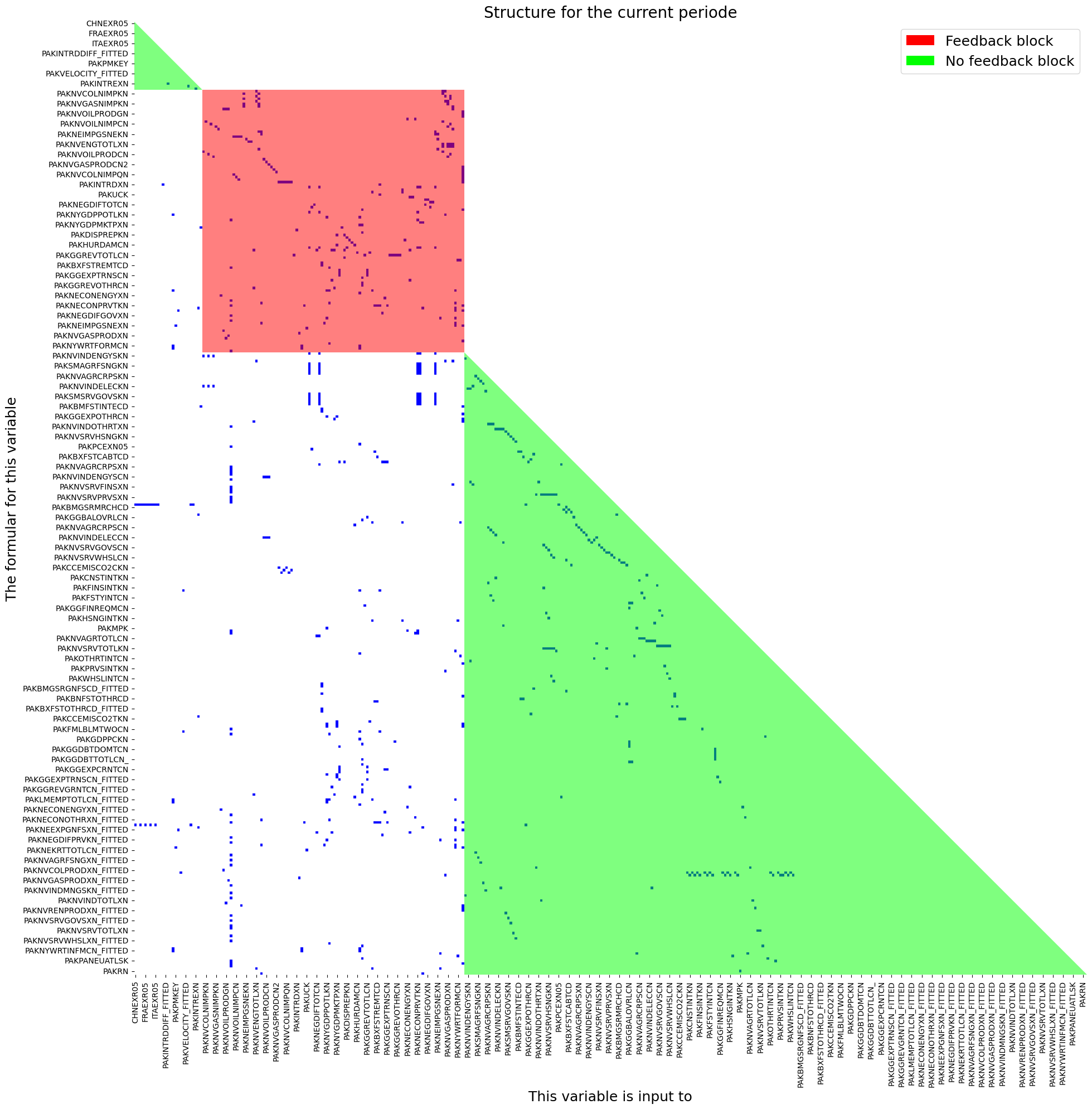
2.13. Model Analytics

When ModelFlow process a model it creates a graph (a network) of the interdependencies between the different variables. The graph is used to find the causal ordering of the model.

A model in MFMod typical contains at least one simultaneous block and a pre and post block.

mpak.plotadjacency(size=(20,20),title='Structure for the current periode');

2.14. Setting time frame

The property .current_per is the master time index for a model instance. It determinate the time frame for simulations and output.

Sometime it can be useful to change the .current_per the property can be set with:

Function	Description
.smpl	Sets the sample period for analysis and reporting.
with .set_smpl:	Sets the sample period for analysis and reporting in a local scope .
with .set_smpl_relative:	Sets the sample period for analysis and reporting relative to the current period or scenario in a local scope.

mpak.current_per

Index([2020, 2021, 2022, 2023, 2024, 2025, 2026, 2027, 2028, 2029, 2030, 2031,
       2032, 2033, 2034, 2035, 2036, 2037, 2038, 2039, 2040, 2041, 2042, 2043,
       2044, 2045, 2046, 2047, 2048, 2049, 2050, 2051, 2052, 2053, 2054, 2055,
       2056, 2057, 2058, 2059, 2060, 2061, 2062, 2063, 2064, 2065, 2066, 2067,
       2068, 2069, 2070, 2071, 2072, 2073, 2074, 2075, 2076, 2077, 2078, 2079,
       2080, 2081, 2082, 2083, 2084, 2085, 2086, 2087, 2088, 2089, 2090, 2091,
       2092, 2093, 2094, 2095, 2096, 2097, 2098, 2099, 2100],
      dtype='int64')

The possible times in the dataframe is contained in the <dataframe>.index property.

mpak.lastdf.index  # the index of the dataframe

Index([1980, 1981, 1982, 1983, 1984, 1985, 1986, 1987, 1988, 1989,
       ...
       2091, 2092, 2093, 2094, 2095, 2096, 2097, 2098, 2099, 2100],
      dtype='int64', length=121)

2.14.1. .smpl, Set time frame

The time frame can be set like this:

mpak.smpl(2020,2025)
mpak.current_per

Index([2020, 2021, 2022, 2023, 2024, 2025], dtype='int64')

2.14.2. .set_smpl, Set timeframe for a local scope

For many operations it can be useful to apply the operations for a shorter time frame, but retain the global time frame after the operation.
This can be done with a with statement like this.

print(f'Global time  before   {mpak.current_per}')
with mpak.set_smpl(2022,2023):
    print(f'Local time frame      {mpak.current_per}')
print(f'Unchanged global time {mpak.current_per}')

Global time  before   Index([2020, 2021, 2022, 2023, 2024, 2025], dtype='int64')
Local time frame      Index([2022, 2023], dtype='int64')
Unchanged global time Index([2020, 2021, 2022, 2023, 2024, 2025], dtype='int64')

2.14.3. .set_smpl_relative Set relative timeframe for a local scope

When creating a script it can be useful to set the time frame relative to the current time.

Like this:

print(f'Global time  before   {mpak.current_per}')
with mpak.set_smpl_relative (-1,0):
    print(f'Local time frame      {mpak.current_per}')
print(f'Unchanged global time {mpak.current_per}')

Global time  before   Index([2020, 2021, 2022, 2023, 2024, 2025], dtype='int64')
Local time frame      Index([2019, 2020, 2021, 2022, 2023, 2024, 2025], dtype='int64')
Unchanged global time Index([2020, 2021, 2022, 2023, 2024, 2025], dtype='int64')

2.15. Reports

ModelFlow offers a range of features to present and visualize model results. Below is a list:

• .table():
  This function creates a table from data in the .lastdf and .basedf dataframes. It can be customized with various arguments to adjust the data type (e.g., growth rate or level), the number of decimals, and table titles.

• .plot():
  This function generates charts based on data from .lastdf, .basedf, or saved scenarios in from .keep_solution. It can be customized with various arguments to choose the chart type, data transformation (e.g., growth rate or level), scenarios to display, and chart titles.

• .text():
  This function creates a text object that can contain plain text, LaTeX code, or HTML code. It is primarily used to add text to reports.

• .report():
  This function combines tables, plots, text, and other reports into a consolidated report. Reports can be saved and reused, making it easy to generate reports for various scenarios.

2.15.1. The .table function

Line Options
These options are set on table creation.

Argument	Default Value	Description
pat	‘#Headline’ (defined in the ModelFlow class)	Variable names to be displayed, may include wildcard specifications.
datatype	‘growth’	Defines the data transformation displays (cf. next table).
mul	1.0	Multiplier of values before display.
dec	2	Set the decimal places to display.
col_desc	Depend on datatype	A centered description of columns (non-transposed table).
heading	‘’	A centered text above columns (non-transposed table).
rename	True	If True, use descriptions; else, use variable names.

Table Options
These options can be revised after a table has been generated.

Argument	Default Value	Description
name	‘’	Name for this display.
custom_description	{}	Custom description, overrides default descriptions.
title	‘’	Title text for the table.
foot	‘’	Footer text for the table.
transpose	False	If True, transposes the table.
chunk_size	0	Specifies the number of columns per chunk in tables.
timeslice	[]	Specifies the time slice for data display.
max_cols	6	Maximum columns when displayed as string.
last_cols	1	In LaTeX, the number of last columns in a display slice.
smpl	(‘’, ‘’)	Set or reset the sample (smpl) for the table.

Table: Data Types and Their Meanings

datatype	Meaning
growth	This is the default setting. Growth rate in percent in the most recent dataset (.lastdf).
level	Values in .lastdf.
gdppct	Percentage of GDP in .lastdf.
qoq_ar	Quarterly growth annualized. - Quarterly models only.
Difference views	``
difgrowth	Change (\(\Delta\)) in growth rates (.lastdf less basedf).
diflevel	Change (\(\Delta\)) in values (.lastdf less basedf).
difgdppct	Change (\(\Delta\)) in the percentage of GDP from (.lastdf less basedf).
difqoq_ar	change in the annualized quarterly growth (.lastdf less basedf)
difpctlevel	Percentage change (\(\Delta\)) in values (.lastdf less basedf).
Values from .basedf	``
basegrowth	Growth rate in percent in .basedf.
baselevel	Level of the data in .basedf
basegdppct	Percentage of GDP in .basedf.
baseqoq_ar	Quarterly growth in .basedf

2.15.2. The .plot function

Line options are set when the plot is created with the .plot() call and can only be set when the object is instantiated.

Argument	Default Value	Description
pat	‘#Headline’	Pattern with wildcard for variable names
datatype	‘growth’	Defines the datatransformation displayes (cf. next table)
mul	1.0	Multiplier of values before display
ax_title_template	‘’	Template for each chart title
by_var	True	Show results by variable (False) or scenario (True)

Plot options can be revised after the plot has been created.

Argument	Default Value	Description
rename	True	If True use descriptions else variable names
scenarios	‘’	Show for .basedf/.lastdf or selected scenarios
name	‘’	Name for this display.
custom_description	{}	Custom description, override default descriptions.
title	‘’	Title (used when samefig=True).
samefig	False	If True, displays all chart in the same plot area.
ncol	2	Number of columns when samefig=True.
size	(10, 6)	Specifies the size of each chart
legend	True	If True, includes a legend in the display.
smpl	(‘’,’’)	set smpl for this plot

The table below summarizes how the combination of datatype and scenarios determines the data displayed in the chart.

Table: Datatype and Scenario Settings

Datatype	scenarios=’’ or omitted	scenarios=’<list of scenarios>’ (Multiple Scenarios)
Value Views
growth (default)	Growth rate (%) in the most recent dataset (.lastdf).	Growth rates for all scenarios.
level	Values from .lastdf.	Values for all scenarios.
gdppct	Percentage of GDP in .lastdf.	Percentage of GDP for all scenarios.
qoq_ar	Quarterly growth (annualized) for quarterly models in .lastdf.	Quarterly growth (annualized) for all scenarios.
Difference Views
difgrowth	Change (\(\Delta\)) in growth rates between .lastdf and .basedf.	Change (\(\Delta\)) in growth rates between the first and other scenarios.
diflevel	Change (\(\Delta\)) in values between .basedf and .lastdf.	Change (\(\Delta\)) in values between the first and other scenarios.
difgdppct	Change (\(\Delta\)) in the percentage of GDP between .basedf and .lastdf.	Change (\(\Delta\)) in the percentage of GDP between the first and other scenarios.
difqoq_ar	Change in quarterly growth (annualized) between .basedf and .lastdf.	Change (\(\Delta\)) in quarterly growth (annualized) between the first and other scenarios.
difpctlevel	Percentage change (\(\Delta\)) in values between .basedf and .lastdf.	Percentage change (\(\Delta\)) in values between the first and other scenarios.
.basedf Views
basegrowth	Growth rate (%) in .basedf.	Growth rates for the first scenario.
baselevel	Values from .basedf.	Values for the first scenario.
basegdppct	Percentage of GDP in .basedf.	Percentage of GDP for the first scenario.
baseqoq_ar	Quarterly growth (annualized) in .basedf.	Quarterly growth (annualized) for the first scenario.

2.15.2.1. .savefigs() Saving plots in other formats.

Plots are created using the matplotlib library. If charts are going to be used further downstream they can be saved to file using a wide range of formats.

.savefigs() options

Parameter	Type	Description	Default
location	str	The folder in which to save the charts.	'./graph'
experimentname	str	A subfolder under location where charts are saved.	'experiment1'
addname	str	An additional name added to each figure filename.	'' (empty string)
extensions	list	A list of file extensions for saving the figures.	['svg']
xopen	bool	If True, open the saved figure locations in a web browser.

Charts can be saved using the following formats:

Extension	Description
.png	Portable Network Graphics
.jpg or .jpeg	t Photographic Experts Group
.tif or .tiff	Tagged Image File Format
.bmp	Bitmap
.gif	Graphics Interchange Format
.svg	Scalable Vector Graphics
.pdf	Portable Document Format
.eps	Encapsulated PostScript
.ps	PostScript
.raw	Raw image data
.rgba	Raw RGBA bitmap
.pgf	Portable Graphics Format

2.15.3. The .text() class

The text class allows the user to define three different types of text: .text_text .html_text and .latex_text. These properties are optional and can be declared explicitly or implicitly.

object	delimited by	contains
.text_text	nothing	Plain text
.html_text	<html> </html>	html text
.latex_text	<latex> </latex>	latex text

2.15.4. Joing plots or tables with |

Tables, Plots can be concatenated together using the | operator. This allows plots or tables with different datatypes to be displayed together.

Plots can only be joined with plots, and tables can only be joined by tables.

2.15.5. Creating reports using + between plots, tables and text

Reports in ModelFlow are containers that can contains figures, plots, tables of different dimension and text. Moreover, Report objects can be saved in a model object and regenerated on new data without requiring any additional effort by the user.

The + operator creates a new report container specification.

Reports can be placed in the dictionary: model instance.reports.Reports can then be reused later.

Functions	task
model instance.add_report(reports,,,)	Add report to model instance.reports, key = report name
model instance.get_report(key)	Returns a report from model instance.reports

A report can be modified with these functions.

Functions	task
.set_scenarios	Set scenarios in report
.set_name	Sets name of report

2.15.6. .set_option() Modifying reports, tables or plots options

With this function options (except line options) can be modified after the element has been created.

2.15.7. Rendering reports, tables, plots and text objects

These objects can be rendered as html, text and pdf objects. The below table indicates the methods associated with each.

Display options for report type objects

command	output
None (just the object name)	In Jupyter Notebook displays the table in its html format.
display(tab)	Displays the table in html format.
.show	Returns a simple text version of the table.
.pdf()	Returns a nicely formatted table in pdf format.

mpak.keep_solutions.keys() 

dict_keys(['Baseline', '$25 increase in oil prices 2025-27', 'Coal, Oil and Gastax : 20', 'Coal, Oil and Gas Carbon tax = 40 USD'])

pat=  ' *NYGDPMKTPKN *NECONPRVTKN  '
tab = mpak.table(pat=pat,name='My_first_table')

pat_gov = '*GGBALOVRLCN *GGDBTTOTLCN *BNCABFUNDCD'
tab_gov = mpak.table(pat_gov,datatype='gdppct',dec=1)
(tab|tab_gov).set_options(smpl=(2022,2026),
    title='{cty_name} GDP components').show

Pakistan GDP components
                                              2022   2023   2024   2025   2026
                                                   --- Percent growth ---     
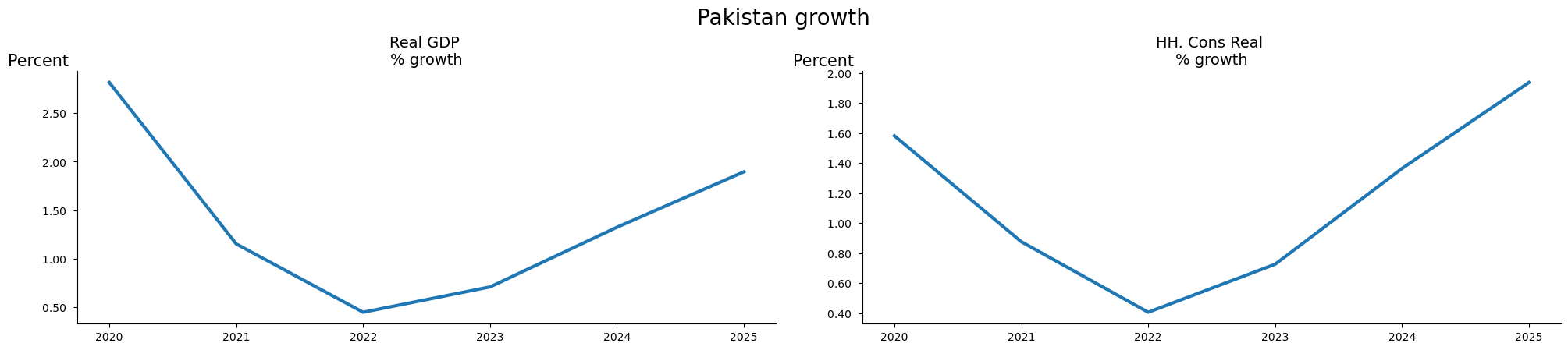
Real GDP                                      0.45   0.71   1.32   1.90   2.32
HH. Cons Real                                 0.41   0.73   1.36   1.94   2.34
                                                   --- Percent of GDP ---     
General Government Revenue, Deficit, LCU mn   -3.5   -3.5   -3.4   -3.3   -3.2
General government gross debt millions lcu    54.9   55.0   55.4   56.0   56.7
Current Account Balance, US$ mn               -4.4   -3.8   -3.5   -3.3   -3.2

fig = mpak.plot(pat,samefig=2,title='{cty_name} growth')
((tab|tab_gov).set_options(smpl=(2022,2026),
    title='{cty_name} GDP components')+fig).show

Pakistan GDP components
                                              2022   2023   2024   2025   2026
                                                   --- Percent growth ---     
Real GDP                                      0.45   0.71   1.32   1.90   2.32
HH. Cons Real                                 0.41   0.73   1.36   1.94   2.34
                                                   --- Percent of GDP ---     
General Government Revenue, Deficit, LCU mn   -3.5   -3.5   -3.4   -3.3   -3.2
General government gross debt millions lcu    54.9   55.0   55.4   56.0   56.7
Current Account Balance, US$ mn               -4.4   -3.8   -3.5   -3.3   -3.2

2.16. Using the index operator .[ ] to select and visualize variables.

Using the index operator on the model instance like this:

mpak[<variable selection>]

will return a special class (called .vis). It implements a number of methods and properties which comes in handy for quick variable:

• vizualization

• analysis

• information

First the user has to select the relevant variables then several properties and methods can be chained

2.16.1. Variable selection

In several contexts it is possible to select a number of variables. Variables can be selected on different basis:

1. Variable name with wildcards

2. Variable descriptions with wildcarts

3. Variable groups

4. all endogenous variables

2.16.1.1. ‘<variable name with wildcards>’… , select matching variables

To select variables the method accept patterns which defines variable names. Wildcards:

• * matches everything

• ? matches any single character

• \[seq] matches any character in seq

• \[!seq] matches any character not in seq

For more how wildcards can be used, the specification can be found here

2.16.1.2. Use of {cty} and deferred substitution in variable selection

Using * or ? to select variables will include all countries, even if some may not be relevant in a particular selection. In order to reuse the same variable selection across different countries deffered substitution can be used.

In this approach, {cty} placeholders can be used. {cty} will be replaced with the ISO 3 letter code for the country in question. And this is done at the execution time - explaining the “deferred” term.

For this to work, a dictionary .substitution must be defined. This dictionary is typically set in the onboarding script but can be set at any point as needed.

Here ???exr05 will select EXR05 for all countries

mpak['???exr05'].names

['CHNEXR05',
 'DEUEXR05',
 'FRAEXR05',
 'GBREXR05',
 'ITAEXR05',
 'PAKEXR05',
 'TUREXR05',
 'USAEXR05']

Here ?only the pakistan value is selected.

If the model is used for another country the cty can be changed, without changing the specification

mpak['{cty}exr05'].names

['PAKEXR05']

2.16.1.3. .substitution Defining deferred substitution

To enable reuse of variable selection and report specification this feature enable substitution of {key} in a string with <model instance>.substitution['key'] where .substitution is a dictionary.

When onboarding a World Bank model the <model instance>.substitution looks like this:

mpak.substitution 

{'cty': 'PAK', 'cty_name': 'Pakistan'}

Deferred substitution works with variable selection, report titles and report text.

mpak['{cty}NYgdpFCSTCN'].endo_nofit.rplot(datatype='growth',
      title='{cty_name} charts',rename=False).show

2.16.1.4. ‘<#Variable group>’ , select variables matching in variable group

2.16.1.5. .var_groups, a dictionary of variable groups

The property .var_groups can contain a dictionary of variables defined by variable names with wildcards.

mpak.var_groups

{'Headline': '{cty}NYGDPMKTPKN {cty}NYGDPMKTPXN {cty}NRTOTLCN {cty}LMUNRTOTLCN {cty}BFFINCABDCD  {cty}BFBOPTOTLCD {cty}GGBALEXGRCN {cty}GGDBTTOTLCN_ {cty}GGDBTTOTLCN {cty}BNCABLOCLCD_ {cty}FPCPITOTLXN {cty}CCEMISCO2TKN',
 'National income accounts': '{cty}NY*',
 'National expenditure accounts': '{cty}NE*',
 'Value added accounts': '{cty}NV*',
 'Balance of payments exports': '{cty}BX*',
 'Balance of payments exports and value added ': '{cty}BX* {cty}NV*',
 'Balance of Payments Financial Account': '{cty}BF*',
 'General government fiscal accounts': '{cty}GG*',
 'World all': 'WLD*',
 'All variables': '*'}

2.16.1.6. Example

mpak['#Balance of payments exports'].des

PAKBXFSTCABTCD        : Exp., Factor Services and Transfers (BOP), US$ mn
PAKBXFSTOTHRCD        : Exp., Other Factor Services and Transfers (BOP), US$ mn
PAKBXFSTOTHRCD_A      : Add factor:Exp., Other Factor Services and Transfers (BOP), US$ mn
PAKBXFSTOTHRCD_D      : Fix dummy:Exp., Other Factor Services and Transfers (BOP), US$ mn
PAKBXFSTOTHRCD_FITTED : Fitted  value:Exp., Other Factor Services and Transfers (BOP), US$ mn
PAKBXFSTOTHRCD_X      : Fix value:Exp., Other Factor Services and Transfers (BOP), US$ mn
PAKBXFSTREMTCD        : Exp., Remittances (BOP), US$ mn
PAKBXFSTREMTCD_A      : Add factor:Exp., Remittances (BOP), US$ mn
PAKBXFSTREMTCD_D      : Fix dummy:Exp., Remittances (BOP), US$ mn
PAKBXFSTREMTCD_FITTED : Fitted  value:Exp., Remittances (BOP), US$ mn
PAKBXFSTREMTCD_X      : Fix value:Exp., Remittances (BOP), US$ mn
PAKBXGSRGNFSCD        : Exp., GNFS (BOP), US$ mn
PAKBXGSRGNFSCD_A      : Add factor:Exp., GNFS (BOP), US$ mn
PAKBXGSRGNFSCD_D      : Fix dummy:Exp., GNFS (BOP), US$ mn
PAKBXGSRGNFSCD_FITTED : Fitted  value:Exp., GNFS (BOP), US$ mn
PAKBXGSRGNFSCD_X      : Fix value:Exp., GNFS (BOP), US$ mn
PAKBXGSRMRCHCD        : Exp., MRCH (BOP), US$ mn
PAKBXGSRMRCHCD_A      : Add factor:Exp., MRCH (BOP), US$ mn
PAKBXGSRMRCHCD_D      : Fix dummy:Exp., MRCH (BOP), US$ mn
PAKBXGSRMRCHCD_FITTED : Fitted  value:Exp., MRCH (BOP), US$ mn
PAKBXGSRMRCHCD_X      : Fix value:Exp., MRCH (BOP), US$ mn
PAKBXGSRNFSVCD        : Exp., NF SERV (BOP), US$ mn

2.16.1.7. ‘<!search pattern>’ , select variables where search pattern with wildcards is matching description

2.16.1.8. .var_descriptions, a dictionary of variable descriptions

The property .var_description contains a dictionary with variable names as key and a description as value.

2.16.1.9. Example

mpak['!*import*'].des

PAKBMFSTINTECD        : Imports, External Debt Interest Payments
PAKNEIMPGNFSKN        : Imports real
PAKNEIMPGNFSKN_A      : Add factor:Imports real
PAKNEIMPGNFSKN_D      : Fix dummy:Imports real
PAKNEIMPGNFSKN_FITTED : Fitted  value:Imports real
PAKNEIMPGNFSKN_X      : Fix value:Imports real
PAKNVCOLNIMPQN        : Coal, net import (ktoe)
PAKNVGASNIMPQN        : Gas, net import (ktoe)
PAKNVOILNIMPQN        : Oil, net import (ktoe)
PAKNVRENNIMPQN        : "Renewables", net import (ktoe)
PAKPMKEY              : Keyfitz Price Imports

2.16.1.10. ‘#ENDO’ , select all edogenous variables

# Show the first 4 names of endogenous variables
mpak['#endo'].names[:4]

['CHNEXR05', 'CHNPCEXN05', 'DEUEXR05', 'DEUPCEXN05']

2.16.2. Access values in .lastdf and .basedf

To limit the output printed, we set the time frame to 2020 to 2023.

mpak.smpl(2020,2023);

To access the values of ‘PAKNYGDPMKTPKN’ and ‘PAKNECONPRVTKN’ from the latest simulation a small widget is displayed.

To access the values of ‘PAKNYGDPMKTPKN’ and ‘PAKNECONPRVTKN’ from the base dataframe, specify .base

mpak['PAKNYGDPMKTPKN PAKNECONPRVTKN'].base.df

	PAKNYGDPMKTPKN	PAKNECONPRVTKN
2020	2.627394e+07	2.367289e+07
2021	2.651137e+07	2.397282e+07
2022	2.668514e+07	2.416413e+07
2023	2.696308e+07	2.442786e+07

2.16.3. .df Pandas dataframe

Sometime you need to perform additional operations on the values. Therefor the .df will return a dataframe with the selected variables.

mpak['PAKNYGDPMKTPKN PAKNECONPRVTKN'].df

	PAKNYGDPMKTPKN	PAKNECONPRVTKN
2020	2.648605e+07	2.338267e+07
2021	2.679140e+07	2.358771e+07
2022	2.691168e+07	2.368379e+07
2023	2.710269e+07	2.385588e+07

2.16.4. .names Variable names

If you select variables using wildcards, then you can access the names that correspond to your query.

mpak['PAKNYGDP??????'].names

['PAKNYGDPDISCCN',
 'PAKNYGDPDISCKN',
 'PAKNYGDPFCSTCN',
 'PAKNYGDPFCSTKN',
 'PAKNYGDPFCSTXN',
 'PAKNYGDPMKTPCD',
 'PAKNYGDPMKTPCN',
 'PAKNYGDPMKTPKD',
 'PAKNYGDPMKTPKN',
 'PAKNYGDPMKTPXN',
 'PAKNYGDPPOTLKN']

2.16.5. .rename() replaces the variable mnemonic with its description

Use .rename() to display results using the variable description instead of the mnemonic, which is the default behavior.

mpak['PAKNYGDPMKTPKN PAKNECONPRVTKN'].rename().df

	Real GDP	HH. Cons Real
2020	2.648605e+07	2.338267e+07
2021	2.679140e+07	2.358771e+07
2022	2.691168e+07	2.368379e+07
2023	2.710269e+07	2.385588e+07

2.16.6. Transformations of solution results

When the variables has been selected through the index operator a number of standard data transformations can be performed.

Transfomation	Meaning	expression
growth (pct)	Growth rates	\(\frac{this_t}{this_{t-1}} -1\)
dif	Difference in level	\(l-b\)
difgrowth (difpct)	Difference in growth rate	\({\big[{\frac{l_t}{l_{t-1}}-1}\big]-\big[{\frac{b_t}{b_{t-1}}-1}\big]}\)
difpctlevel	difference in level as a pct of baseline	\(\frac{l_t-b_t}{b_t} \)

• \(this\) is the chained value. Default lastdf but if preceeded by .base the values from .basedf will be used

• \(b\) is the values from .basedf

• \(l\) is the values from .lastdf

2.16.7. .dif Difference in level

The ‘dif’ command displays the difference in levels of the latest and previous solutions.

\(l-b\)

where l is the variable from the .lastdf and b is the variable from .basedf.

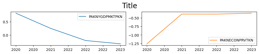
mpak['PAKNYGDPMKTPKN PAKNECONPRVTKN'].dif.plot()

2.16.8. .growth (.pct) Growth rates

Display growth rates

\(\left(\cfrac{l_t}{l_{t-1}}-1\right )\)

mpak['PAKNYGDPMKTPKN PAKNECONPRVTKN'].growth.plot();

2.16.9. .difpct property difference in growth rates

The difference in the growth rates between the last and base dataframe.

\(\left( \cfrac{l_t}{l_{t-1}}-1 \right) - \left(\cfrac{b_t}{b_{t-1}}-1 \right)\)

mpak['PAKNYGDPMKTPKN PAKNECONPRVTKN'].difpct.plot() ; 

2.16.10. .difpctlevel percent difference of levels

\(\left( \cfrac{l_t-b_t}{b_{t}} \right) \)

mpak['PAKNYGDPMKTPKN PAKNECONPRVTKN'].difpctlevel.plot();  

2.16.11. .yoy_ar Growth over 4 periods

This should only be used for quarterly data

\(\left( \cfrac{l_t-b_{t-4}}{b_{t-4}} \right)-1 \)

2.16.12. .qoq_ar Annualized quarterly growth rate

Also for quarterly data

\(\left( \cfrac{l_t-b_t}{b_{t}} \right)^4-1 \)

2.17. .plot chart the selected and transformed variables

After the variables has been selected and transformed, they can be plotted. The .plot() method plots the selected variables separately

mpak.smpl(2020,2100);

mpak['PAKNYGDP??????'].rename().plot(title="A wild card selection");

2.17.1. Options to plot()

Common:

• title (optional): title. Defaults to ‘’.

• colrow (TYPE, optional): Columns per row . Defaults to 2.

• sharey (TYPE, optional): Share y axis between plots. Defaults to False.

More excotic:

• splitchar (TYPE, optional): If the name should be split . Defaults to ‘__’.

• savefig (TYPE, optional): Save figure. Defaults to ‘’.

• xsize (TYPE, optional): x size default to 10

• ysize (TYPE, optional): y size per row, defaults to 2

• ppos (optional): # of position to use if split. Defaults to -1.

• kind (TYPE, optional): Matplotlib kind . Defaults to ‘line’.

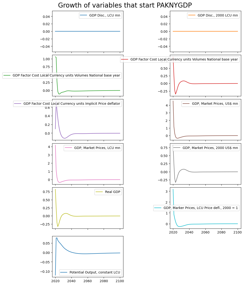
mpak['PAKNYGDP??????'].difpct.rename().plot(title='Growth of variables that start PAKNYGDP');

2.18. [].rtable and [].rplot - reports from []

Report tables and plots can also be created directly from the variable selector []. The purpose is to enable easy reuse of variable selection.

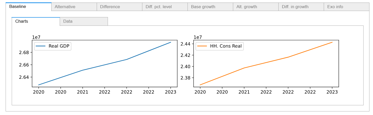
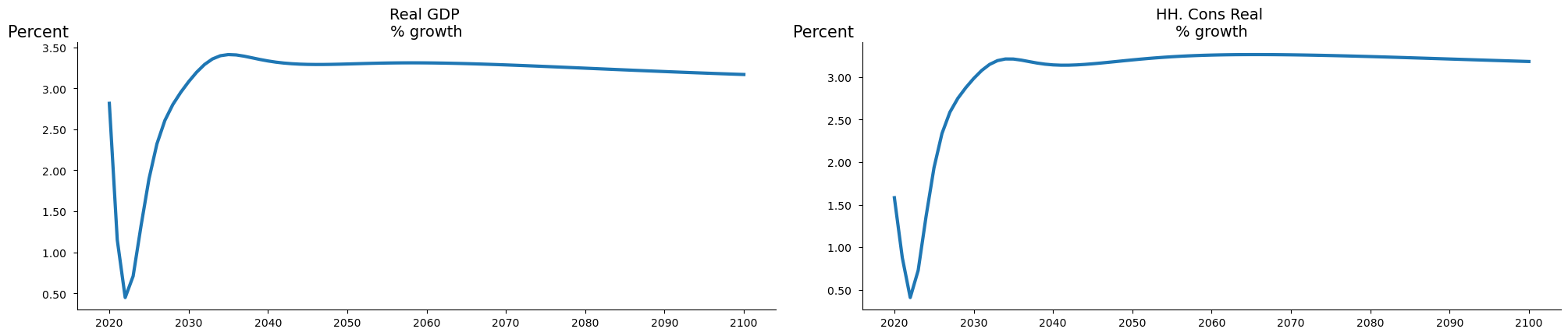
mpak['PAKNYGDPMKTPKN PAKNECONPRVTKN'].rplot(samefig=1).show 

2.19. Plotting inspiration

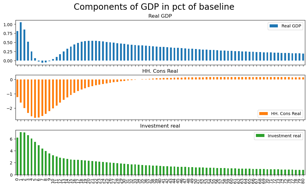
The following graph shows the components of GDP using the values of the baseline dataframe.

mpak['PAKNYGDPMKTPKN PAKNECONPRVTKN PAKNEGDIFTOTKN'].\
difpctlevel.rename().\
plot(title='Components of GDP in pct of baseline',colrow=1,kind='bar') ;

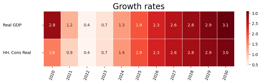
2.19.1. Heatmaps

For some model types heatmaps can be helpful, and they come out of the box. This feature was developed for use by bank stress test models.

with mpak.set_smpl(2020,2030):
    mpak['PAKNYGDPMKTPKN PAKNECONPRVTKN'].pct.rename().heat(title='Growth rates',annot=True,dec=1,size=(10,3))  

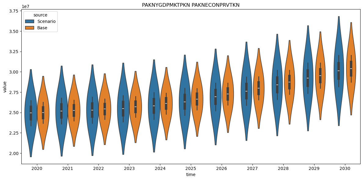
2.19.2. Violin and boxplots,

Not obvious for macro models, but useful for stress test models with many banks.

with mpak.set_smpl(2020,2030): 
    mpak['PAKNYGDPMKTPKN PAKNECONPRVTKN'].difpct.box()  
    mpak['PAKNYGDPMKTPKN PAKNECONPRVTKN'].difpct.violin()  

2.19.3. Plot baseline vs alternative

A raw routine, only showing levels. To make it really useful it should be expanded.

mpak['PAKNYGDPMKTPKN PAKNECONPRVTKN'].plot_alt() ;

2.20. .draw() Graphical presentation of relationships between variables

.draw() helps you understand the relationship between variables in your model better.

The thickness the arrow reflect the attribution of the upstream variable to the impact on the downstream variable.

2.20.1. .draw(up = level, down = level)

You can specify how many levels up and down you want in your graphical presentation (Needs more explanation).

In this example all variables that depend directly upon GDP and consumption as well as those that are determined by them, are displayed. This means one step upstream in the model logic and one step downstream.

More on the how to visualize the logic structure here

mpak['PAKNYGDPMKTPKN PAKNECONPRVTKN'].draw(up=1,down=1,png=latex)  # diagram of all direct dependencies 

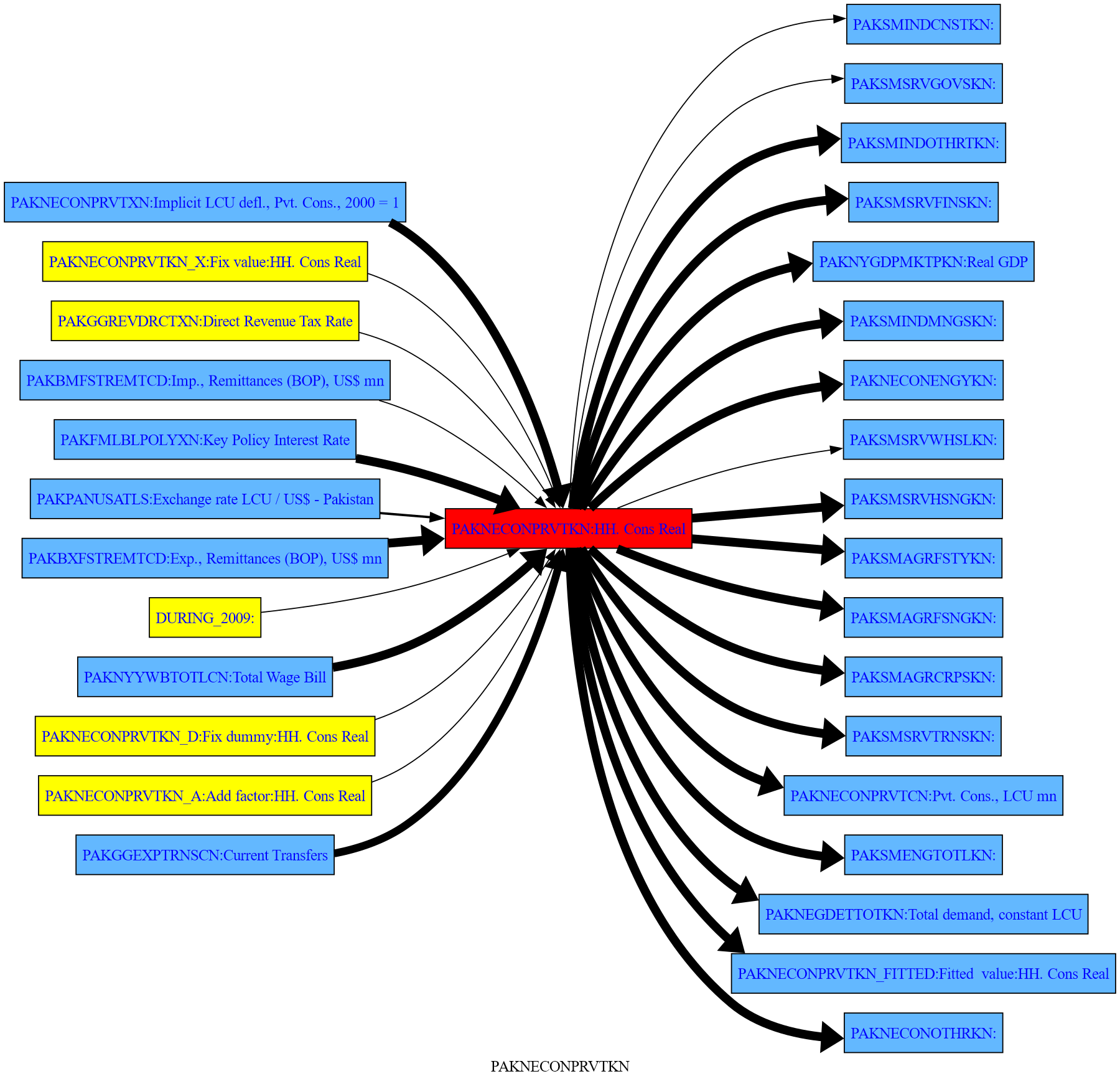
2.20.2. .draw(filter =<minimal impact>)

By specifying filter= only links where the minimal impact is more than <minimal impact> are show. In this case 20%

mpak['PAKNECONPRVTKN'].draw(up=3,down=1,filter=20,png=latex)  

2.21. Attribution/decomposition

Attribution is about taking the total derivative of a function. This can be done at two levels:

• single equation To investigate the impact of changes in right hand variables on the left hand variables

• model To investigate the impact of changes in exogenous variables on selected endogenous variables

2.21.1. Single equations attribution

This can either be done where the changes in variables are between:

• A baseline and an alternative (usualy .basedf and .lastdf (default)

• From year to year.

2.21.1.1. .dekomp() Attribution of right hand side variables to change in left hand side.

The .dekomp() function is the engine for calculates the contributions of the right hand side variables to the observed change in the left hand side variables.

The user will usual benefit from using some of the wrappers which can display the results of .dekomp()

Parameter	Description
varnavn	Input variable name.
start	Start period for retrieving variable values (default is ‘’).
end	End period for retrieving variable values (default is ‘’).
basedf	Base dataframe to use (default is None, meaning ‘.basedf’).
altdf	Alternative dataframe to use (default is None, meaning .lastdf).
lprint	Flag to print the results (default is True).
time_att	Flag to do a timewise attribute (default is False).

.dekomp() returns a named tupple with the results as Dataframes.

Field	Meaning
diff_level	DataFrame with level differences.
att_level	DataFrame with attributions to the level difference.
att_pct	DataFrame with the share of attributions to the difference in level.
diff_growth	DataFrame with differences in growth rate.
att_growth	DataFrame with attributions to the difference in growth rate. (not accurate)

mpak.dekomp.cache_clear()
with mpak.set_smpl(2021,2022):
    dekomp_result = mpak.dekomp('PAKNYGDPMKTPKN',lprint=1)  # frml attribution 

Formula        : FRML <IDENT> PAKNYGDPMKTPKN = PAKNECONPRVTKN+PAKNECONGOVTKN+PAKNEGDIFTOTKN+PAKNEGDISTKBKN+PAKNEEXPGNFSKN-PAKNEIMPGNFSKN+PAKNYGDPDISCKN+PAKADAP*PAKDISPREPKN $ 

                       2021        2022
Variable    lag                        
Base        0   26511370.45 26685141.90
Alternative 0   26791399.30 26911678.26
Difference  0     280028.85   226536.36
Percent     0          1.06        0.85

 Contributions to difference for  PAKNYGDPMKTPKN
                         2021       2022
Variable       lag                      
PAKNECONPRVTKN 0   -385108.31 -480338.16
PAKNECONGOVTKN 0    348838.85  308073.15
PAKNEGDIFTOTKN 0    218058.91  217582.81
PAKNEGDISTKBKN 0        -0.02      -0.01
PAKNEEXPGNFSKN 0     -3355.88   -6206.24
PAKNEIMPGNFSKN 0    101595.21  187424.78
PAKNYGDPDISCKN 0        -0.02      -0.01
PAKADAP        0        -0.02      -0.01
PAKDISPREPKN   0        -0.02      -0.01

 Share of contributions to difference for  PAKNYGDPMKTPKN
                         2021       2022
Variable       lag                      
PAKNECONGOVTKN 0         125%       136%
PAKNEGDIFTOTKN 0          78%        96%
PAKNEIMPGNFSKN 0          36%        83%
PAKNEGDISTKBKN 0          -0%        -0%
PAKNYGDPDISCKN 0          -0%        -0%
PAKADAP        0          -0%        -0%
PAKDISPREPKN   0          -0%        -0%
PAKNEEXPGNFSKN 0          -1%        -3%
PAKNECONPRVTKN 0        -138%      -212%
Total          0         100%       100%
Residual       0          -0%        -0%

 Difference in growth rate PAKNYGDPMKTPKN
                      2021       2022
Variable    lag                      
Base        0         0.9%       0.7%
Alternative 0         1.2%       0.4%
Difference  0         0.2%      -0.2%
None

 Contribution to growth rate PAKNYGDPMKTPKN
                         2021       2022
Variable       lag                      
PAKNECONPRVTKN 0        -0.3%      -0.3%
PAKNECONGOVTKN 0         0.1%      -0.2%
PAKNEGDIFTOTKN 0         0.1%      -0.0%
PAKNEGDISTKBKN 0         0.0%       0.0%
PAKNEEXPGNFSKN 0        -0.0%      -0.0%
PAKNEIMPGNFSKN 0         0.4%       0.3%
PAKNYGDPDISCKN 0         0.0%       0.0%
PAKADAP        0         0.0%       0.0%
PAKDISPREPKN   0         0.0%       0.0%
Total          0         0.3%      -0.2%
Residual       0         0.0%       0.0%

The content of the returned namedtupple

for name, value in dekomp_result._asdict().items():
    print(f"{name}:\n {value}")

diff_level:
                             2021             2022
Variable    lag                                  
Base        0    26511370.451597  26685141.900638
Alternative 0    26791399.301257  26911678.264054
Difference  0      280028.849661    226536.363416
Percent     0           1.056259         0.848923
att_level:
                              2021           2022
Variable       lag                              
PAKNECONPRVTKN 0   -385108.305552 -480338.157967
PAKNECONGOVTKN 0    348838.846058  308073.148036
PAKNEGDIFTOTKN 0    218058.909007  217582.809019
PAKNEGDISTKBKN 0        -0.017471       -0.00759
PAKNEEXPGNFSKN 0     -3355.878372   -6206.242849
PAKNEIMPGNFSKN 0    101595.208089  187424.776355
PAKNYGDPDISCKN 0        -0.017471       -0.00759
PAKADAP        0        -0.017471       -0.00759
PAKDISPREPKN   0        -0.017471       -0.00759
att_pct:
                           2021        2022
Variable       lag                        
PAKNECONGOVTKN 0    124.572467  135.992802
PAKNEGDIFTOTKN 0     77.870158   96.047630
PAKNEIMPGNFSKN 0     36.280265   82.734963
PAKNEGDISTKBKN 0     -0.000006   -0.000003
PAKNYGDPDISCKN 0     -0.000006   -0.000003
PAKADAP        0     -0.000006   -0.000003
PAKDISPREPKN   0     -0.000006   -0.000003
PAKNEEXPGNFSKN 0     -1.198405   -2.739623
PAKNECONPRVTKN 0   -137.524511 -212.035786
Total          0     99.999950   99.999973
Residual       0     -0.000050   -0.000027
diff_growth:
                      2021      2022
Variable    lag                    
Base        0    0.903664  0.655460
Alternative 0    1.152860  0.448946
Difference  0    0.249196 -0.206514
att_growth:
                             2021          2022
Variable       lag                            
PAKNECONPRVTKN 0   -3.418828e-01 -3.440505e-01
PAKNECONGOVTKN 0    9.539784e-02 -1.600896e-01
PAKNEGDIFTOTKN 0    1.061517e-01 -5.475665e-03
PAKNEGDISTKBKN 0    5.848919e-08  3.717548e-08
PAKNEEXPGNFSKN 0   -8.896135e-03 -1.058154e-02
PAKNEIMPGNFSKN 0    4.020092e-01  3.198729e-01
PAKNYGDPDISCKN 0    5.848919e-08  3.717548e-08
PAKADAP        0    5.848919e-08  3.717548e-08
PAKDISPREPKN   0    5.848919e-08  3.717548e-08
Total          0    2.527800e-01 -2.003243e-01
Residual       0    3.584398e-03  6.189603e-03

2.21.1.2. Useful wrappers of single equation attribution

Command	Explanation
Variable attribution
<modelinstance>.<variable name>.dekomp()	Perform a decomposition analysis for the variable.
<modelinstance>[pattern].dekomp()	Perform decomposition analysis on variables matching the given pattern.
Attribution Extraction	Use threshold=<number>to limit small attributions
<modelinstance>.get_att_pct('<variable name>')	Get the percentage attribution for the variable.
<modelinstance>.get_att_level('<variable name>')	Get the level attribution for the variable.
Plotting attribution	Use threshold=<number>to limit small attributions
<modelinstance>.dekomp_plot('<variable name>')	Plot the decomposition analysis results for the variable.
<modelinstance>.dekomp_plot_per('<variable name>')	Plot decomposition results for a specific period for the variable.
<modelinstance>.get_dekom_gui('<variable name>')	Display an interactive GUI for performing decomposition analysis.
Enhance causal graph with attribution	Use filter=<percent number> to prune causality graph
<modelinstance>.<variable name>.draw()	Generate a visual representation of the variable’s relationships.
<modelinstance>.<variable name>.tracepre()	Trace the predecessors of the variable to understand upstream dependencies.
<modelinstance>.<variable name>.tracedep()	Trace the dependents of the variable to understand downstream effects.
<modelinstance>.modeldash('<variable name>')	Display an interactive dashboard for analyzing the variable.

2.21.2. Model Attribution

The method .totdif() returns an instance of the totdif class.

It works by solving the model multiple times, each time modifying one of the right-hand side variables and calculating the impact on all dependent variables. By default, it uses the values from the .lastdf DataFrame as the shock values and the values in .basedf as the baseline (initial) values. Separate simulations are run for every exogenous (or exogenized) variable that has changed between the two DataFrames.

For advanced users, the right-hand side (RHS) variables can be grouped into user-defined blocks. This feature is particularly useful when there are many changes, as it helps identify the primary causal pathways.

The result of the attribution analysis is stored in the .res property of the totdif class instance. This property contains a dictionary with two keys: 'level' and 'growth'. These represent the impacts of each exogenous variable or group on the level and growth metrics, respectively.

The totdif class also provides several methods to display the results of the attribution analysis. This eliminates the need to directly access the .res property unless custom output is required beyond the standard visualizations.

2.21.2.1. The .totdif() Method

In most cases, there is no need to provide parameters to this method. However, if a model is very large, it can be useful to limit the number of variables included in the analysis. This can be controlled using the summaryvar parameter.

In certain circumstances, it can also be helpful to group exogenous variables into categories that are analyzed as a whole. For example, in a model with many countries, it might make sense to group shocks by country. Alternatively, it could be useful to group shocks by type across all countries. This grouping can be achieved by setting the experiments parameter.

Parameter	Type	Description	Default
summaryvar	str or list	Variables to summarize in the analysis. Use '*' to include all variables.	'*'
experiments	dict	A dictionary where keys are experiment names and values are lists of variables to reset to baseline values. If None, uses all variables with differences.	None

totdekomp = mpak.totdif() # Calculate the total derivative½s of all equations in the model.

Total dekomp took       :         3.728 Seconds

totdekomp.res.keys() 

dict_keys(['level', 'growth'])

2.21.2.2. .totexplain() to display the results

Parameter	Type	Description	Default
pat	str	Pattern to match variables for attribution analysis.	'*'
vtype	str	Type of data to attribute. Options: 'all', 'per', 'last', 'sum'.	'all'
stacked	bool	Whether to stack the data in the visualization (relevant for bar or area plots).	True
kind	str	Type of plot to generate. Options: 'bar', 'line', 'area', etc.	'bar'
per	str or int	Specific period to analyze (used when vtype is 'per').	'' (empty)
title	str	Title for the plot. If empty, a default title will be generated based on the analysis type.	'' (empty)
use	str	Type of decomposition to use. Options: 'level', 'growth'.	'level'
threshold	float	Minimum impact value to include in the visualization (filters out smaller impacts).	0.0
ysize	int	Height of the plot in inches.	10
**kwargs	dict	Additional keyword arguments passed to underlying visualization methods.	N/A

The meaning of vtype is:

vtype Value	Description
'all'	Performs attribution analysis across all periods and provides a complete decomposition overview.
'per'	Analyzes and visualizes the decomposition for a specific period.
'last'	Focuses on the decomposition of the last period in the data.
'sum'	Summarizes and visualizes the cumulative impact across all periods.

totdekomp.totexplain('PAKNYGDPMKTPKN',kind='area',stacked=True);

2.22. Bespoken plots using matplotlib (or plotly -later) (should go to a separate plot book

The predefined plots are not necessary created for presentation purpose. To create bespoken plots they can be constructed directly in python scripts. The two main libraries are matplotlib, plotly but any ther python plotting library can be used. Here is an example using matplotlib.

2.23. Plot four separate plots of multiple series in grid

figure,axs= plt.subplots(2,2,figsize=(11, 7))
axs[0,0].plot(mpak.basedf.loc[2020:2099,'PAKGGBALOVRLCN_'],label='Baseline')
axs[0,0].plot(mpak.lastdf.loc[2020:2099,'PAKGGBALOVRLCN_'],label='Scenario')
#axs[0,0].legend()

axs[0,1].plot(mpak.basedf.loc[2020:2099,'PAKGGDBTTOTLCN_'],label='Baseline')
axs[0,1].plot(mpak.lastdf.loc[2020:2099,'PAKGGDBTTOTLCN_'],label='Scenario')

axs[1,0].plot(mpak.basedf.loc[2020:2099,'PAKGGREVTOTLCN']/mpak.basedf.loc[2020:2099,'PAKNYGDPMKTPCN']*100,label='Baseline')
axs[1,0].plot(mpak.lastdf.loc[2020:2099,'PAKGGREVTOTLCN']/mpak.lastdf.loc[2020:2099,'PAKNYGDPMKTPCN']*100,label='Scenario')

axs[1,1].plot(mpak.basedf.loc[2020:2099,'PAKGGREVGRNTCN']/mpak.basedf.loc[2020:2099,'PAKNYGDPMKTPCN']*100,label='Baseline')
axs[1,1].plot(mpak.lastdf.loc[2020:2099,'PAKGGREVGRNTCN']/mpak.lastdf.loc[2020:2099,'PAKNYGDPMKTPCN']*100,label='Scenario')
#axs2[4].plot(mpak.lastdf.loc[2000:2099,'PAKGGREVGRNTCN']/mpak.basedf.loc[2000:2099,'PAKNYGDPMKTPCN']*100,label='Scenario')

axs[0,0].title.set_text("Fiscal balance (% of GDP)")
axs[0,1].title.set_text("Gov't Debt (% of GDP)")
axs[1,0].title.set_text("Total revenues (% of GDP)")
axs[1,1].title.set_text("Grant Revenues (% of GDP)")
figure.suptitle("Fiscal outcomes")

plt.figlegend(['Baseline','Scenario'],loc='lower left',ncol=5)  
figure.tight_layout(pad=2.3) #Ensures legend does not overlap dates
figure

---

[1]

For those familiar with programming in Python, technically this is implemented as the model class method __call__.