1. Introduction to Jupyter Notebook#
Jupyter Notebook is an application for creating, annotating, simulating and working with computational documents. Originally developed for python, the latest versions of EViews also support Jupyter Notebooks.
Jupyter Notebook offers a simple, streamlined, document-centric experience and can be a great environment for documenting the work you are doing, and trying alternative methods of achieving desired results. Many of the methods in ModelFlow have been developed to work well with Jupyter Notebook. Indeed this documentation was written as a series of Jupyter Notebooks bound together with the Jupyter Book package.
Jupyter Notebook is not the only way to work with ModelFlow or Python. As users become more advanced they are likely to migrate to a more program-centric IDE (Interactive Development Environment) like Spyder or Microsoft Visual Code.
However, to start, Jupyter Notebooks is a great environment in which to follow work done by others, try out code, and tweak the codes of others to fit your own needs.
In this chapter - Introduction to Jupyter Notebook
This chapter introduces Jupyter Notebook. It can be safely skipped by readers already familiar with Jupyter Notebook (an interactive environment for programming, documenting, and analyzing data).
Key points in the chapter include:
What is Jupyter Notebook:
A tool for creating and sharing computational documents that integrate code, text, and visualizations.
Ideal for prototyping, debugging, and documenting workflows.
Getting Started:
Activate the Python environment and launch Jupyter Notebook from the command line.
Navigate to your desired working directory and start a new notebook.
Notebook Structure:
Composed of cells that can contain code, markdown, or outputs.
Cells have two modes: Edit (for writing code or text) and Command (for running cells or managing notebook structure).
Key Features:
Write and execute Python code interactively.
Use Markdown for formatted text, including headers, bullet points, and inline mathematics.
Render complex mathematical equations with LaTeX.
Shortcuts and Tips:
Use keyboard shortcuts to navigate, edit, and execute cells efficiently.
Combine code, results, and documentation in one notebook for replicability.
There are many fine tutorials on Jupyter Notebook on the web, and The official Jupyter site is a good starting point. Another good reference is here.
The remainder of this chapter aims to provide enough information to get a user started.
1.1. Starting Jupyter Notebook#
Each time, a user wants to work with ModelFlow, they will need to activate the ModelFlow environment by
Opening the Anaconda command prompt window (Windows Start->Type Anaconda->Select Anaconda Command Prompt)
Activate the
ModelFlowenvironment we just created by executing the following command:conda activate ModelFlowNavigate to a position on his/her computer’s directory structure where they want to store (or where they are already stored) their
Jupyter Notebooks. (e.g. cd c:\users\MyUserName\MyJupyterNotebookDirectory)Finally, the
Jupyter Notebookpython program must be started by executing the following command from the conda command line:
jupyter notebook
This will launch the Jupyter environment in your default web browser, which should look something like the image below, where the directory structure presented is that of the directory from which the jupyter notebook command was executed (e.g. c:\users\MyUserName\MyJupyterNotebookDirectory).
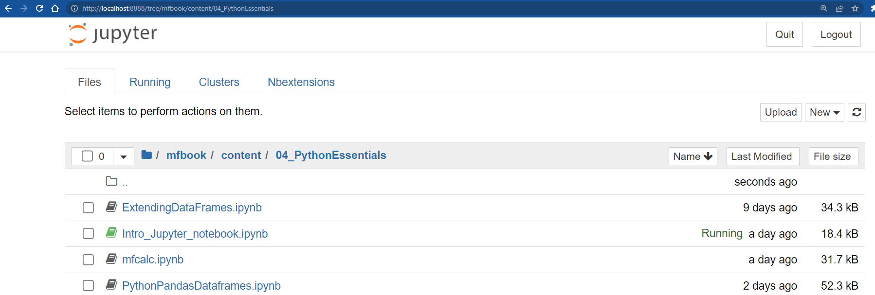
Fig. 1.1 The Jupyter File explorer view#
Warning
Note the directory from which you execute the jupyter notebook will be the root directory for the jupyter session. Only directories and files below this root directory will be accessible by Jupyter.
1.2. Creating a notebook#
The idea behind Jupyter Notebook is to create an interactive version of the physical notebooks that scientists use(d) to:
record what they have done
perhaps explain why
document how data were generated, and
record the results of their experiments
The motivation for these notebooks and Jupyter Notebook is to record the precise steps taken to produce a set of results, which, if followed, would allow others to generate the same results.
To create a new blank notebook you must select from the Jupyter Notebook menu
File-> New Notebook
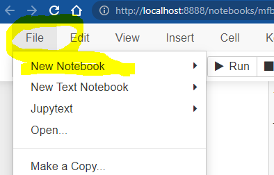
Fig. 1.2 A newly created Jupyter Notebook session#
This will generate a blank unnamed notebook with one empty cell, that looks something like this:
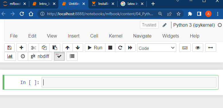
Fig. 1.3 A newly created Jupyter Notebook#
Note
Each notebook has associated with it a “Kernel”, which is an instance of the computing environment in which code will be executed. For Jupyter Notebooks that work with ModelFlow this will be a python Kernel. If your computer has more than one “kernel” installed on it, you may be prompted when creating a new notebook for the kernel with which to associate it. Typically this should be the Python Kernel under which your ModelFlow was built – currently python 3.13 in June 2025.
1.3. Jupyter Notebook cells#
A Jupyter Notebook is comprised of a series of cells.
Jupyter Notebook cells can contain:
computer code: typically python code, but, as noted, other kernels – like EViews – can also be used with
Jupyter.markdown text: plain text that can include special characters that make some text appear as bold, or indicate the text is a header, or instruct
Jupyterto render the text as a mathematical formula. All of the text in this document was entered usingJupyter Notebook’s markdown language (more on this below).Results (in the form of tables or graphs) from the execution of computer code specified in a code cell.
Every cell has two modes:
Edit mode – indicated by a green vertical bar. In edit mode, the user can change the code, or the markdown.
Command mode – indicated by a blue vertical bar. This will be the state of the cell when its content has been executed. For markdown cells this means that the text and special characters have been rendered into formatted text. For code cells, this means the code has been executed and its output (if any) is displayed in an output cell that will be generated in the space immediately below the code cell that generated the output. Also the keyboard is mapped to actions which allows the user to perform tasks like selecting and copying on the cells.
Users can switch between Edit and Command Mode by hitting Esc (to Command mode) or Enter (to Edit mode). With the mouse a double-click in the cell content will switch to Edit Mode and a click in the cell margin will switch to the Command mode.
```{note} Jupyter Notebooks were designed to facilitate replicability: the idea that a scientific analysis should contain - in addition to the final output (text, graphs, tables) - all the computational steps needed to get from raw input data to the results.
1.3.1. How to add, delete and move cells#
The newly created Jupyter Notebook will have a code cell by default. Cells can be added, deleted and moved either via mouse using the toolbar or by keyboard shortcut.
Using the Toolbar
+ button: add a cell below the current cell
scissors: cut current cell (can be undone from “Edit” tab)
clipboard: paste a previously cut cell to the current location
arrows (up and down): move cells (cell must be in Select/Copy mode – vertical side bar must be blue)
hold shift + click cells in left margin: select multiple cells (vertical bar must be blue)
Using keyboard short cuts
esc + a: add a cell above the current cell
esc + b: add a cell below the current cell
esc + d+d: delete the currently selected cell(s)
1.3.2. Change the type of a cell#
You can also change the type of a cell. New cells are by default “code” cells.
Using the Toolbar
Select the desired type from the drop down. options include
Markdown
Code
Raw NBConvert
Using keyboard short cuts
esc + m: make the current cell a markdown cell
esc + y: make the current cell a code cell
Auto-complete and context-sensitive help
When editing a code cell, you can use these short-cuts to autocomplete and or call up documentation for a command.
tab: autocomplete and method selection
double tab: documentation (double tab for full doc)
1.3.3. Execution of cells#
Every cell in a Jupyter Notebook can be executed. Executing a markdown cell will cause the cell’s content to be rendered as html. Executing a python code cell, will cause its content to be executed. Cells can be executed either by using the Run button on the Jupyter Notebook menu, or by using one of two keyboard shortcuts:
ctrl + Enter: Executes the code in the cell or formats the markdown of a cell. The current cell retains the focus. The cursor will stay on the cell that was executed.
shift + enter: Executes the code in the cell or formats the markdown of a cell. The focus (cursor) jumps to the next cell.
For other useful shortcuts see “Help” => “Keyboard Shortcuts” or simply press the keyboard icon in the toolbar.
1.3.3.1. Executing python code#
Below is a code cell with some standard python that declares a variable “x”, assigns it the value 10, declares a second variable “y” and assigns it the value 45. The final line of y alone, instructs python to display the value of the variable y. The results of the operation appear in Jupyter Notebook as an output cell Out[#]. By pressing Ctrl-Enter the code will be executed and the output displayed below.
x = 10
y = 45
y
45
The semi-colon “;” suppresses output in Jupyter Notebook
In the example below, a semi-colon “;” has been appended to the final line. This suppresses the display of the value contained by y; As a result there is no output cell.
x = 10
y = 45
y;
Another way to display results is to use the print function. In this instance even if there is a semicolon at the end of the line, the result of the print command is still output.
x = 10
print(x);
10
Variables in a Jupyter Notebook session are persistent, as a result in the subsequent cell, we can declare a variable ‘z’ equal to 2*y and it will have the value 90.
z=y*2
z
90
The natural order is to execute them sequentially in the order they appear in the Jupyter Notebook. However, when debugging or developing code it may be useful to execute cells out of their natural order.
The persistence of data (the fact that a variable y defined in one cell can be used in another cell) depends on the order in which cells were executed, not the order they appear in the notebook.
1.3.4. Markdown cells and the markdown scripting language in Jupyter Notebook#
Text cells in a notebook can be made more interesting by using markdown.
Cells designated as markdown cells when executed are rendered in a rich text format (html).
Markdown is a lightweight markup language for creating formatted text using a plain-text editor. Used in a markdown cell of Jupyter Notebook it can be used to produce nicely formatted text that mixes text, mathematical formulae, code and outputs from executed python code.
Rather than the relatively complex commands of html <h1></h1>, markdown uses a simplified set of commands to control how text elements should be rendered.
1.3.4.1. Common markdown commands#
Some of the most common of these include:
symbol |
Effect |
|---|---|
# |
Header |
## |
second level |
### |
third level etc. |
**Bold text** |
Bold text |
*Italics text* |
Italics text |
* text |
* Bulleted text or dot notes |
1. text |
1. Numbered bullets |
1.3.4.2. Tables in markdown#
Tables like the one above can be constructed using the symbol | as a separator.
Below is the markdown code that generated the above table:
| symbol           | Effect          |
|:--|:--|                                # Specifies the justification for the columns of the table.
| \#               | Header        |
| \#\#             | second level |
| \*\*Bold text\*\* | **Bold text**   |
| \*Italics text\* | *Italics text*   |
|
| 1\. text  | 1. Numbered bullets   |
The |:–|:–| on the second line tells the Table generator how to justify the contents of columns. The \ before the #s above tells markdown to ignore the normal meaning of # and just show the symbol.
Symbol |
Meaning |
|---|---|
|
left justify |
|
center justify |
|
right justify. |
|
Literal operator. Display what follows do not interpret it in the normal way. |
1.3.4.3. Displaying code#
To display a block of (unexecutable) code within a markdown cell, encapsulate it (surround it) with backticks `.
1.3.4.3.1. Inine code blocks#
For inline code references ‘ a single back tick at the beginning and end suffices. For example, the below line
An example sentence with some back-ticked `text as code` in the middle will render as:
An example sentence with some back-ticked text as code in the middle.
1.3.4.3.2. Multiline code block#
For a multiline section of code use three backticks at the beginning and end.
The below block of code:
```
Multi line
text to be rendered as code
```
will render as:
Multi line
text to be rendered as code
1.3.4.4. Rendering mathematics in markdown#
Jupyter Notebook’s implementation of Markdown supports latex mathematical notation.
Maths can be displayed either inline – surrounded by non mathematical text on the same line, or as a standalone equation.
Below is an example of inline mathematics, which was generated by surrounding the latex maths expression by the $ sign:
The inline code $y_t = \beta_0 + \beta_1 x_t + u_t\$ will renders as: \(y_t = \beta_0 + \beta_1 x_t + u_t\)
if enclosed in $$ $$ the encapsulated javascript will render on its own line.
$$y_t = \beta_0 + \beta_1 x_t + u_t$$
will be rendered centered on its own line – as here.
1.3.4.5. Complex and multi-line math#
Multiline expressions and equations can also be rendered:
\begin{align*}
Y_t  &=  C_t+I_t+G+t+ (X_t-M_t) \\
C_t &= c(C_{t-1},C_{t-2},I_t,G_t,X_t,M_t,P_t)\\
I_t &= i(I_{t-1},I_{t-2},C_t,G_t,X_t,M_t,P_t)\\
G_t &= g(G_{t-1},G_{t-2},C_t,I_t,X_t,M_t,P_t)\\
X_t &= x(X_{t-1},X_{t-2},C_t,I_t,G_t,M_t,P_t,P^f_t)\\
M_t &= m(M_{t-1},M_{t-2},C_t,I_t,G_t,X_t,P_t,P^f_t)
\end{align*}
The above latex mathematics code uses the & symbol to tell latex to align the different lines (separated by \\) on the character immediately after the &. In this instance the equals “=” sign. The * after align supresses equation numbering.
1.3.5. links to more info on markdown#
There are many very good markdown cheatsheets and tutorials on the internet, one cheatsheet can be found here.