7. Report writing and scenario results

ModelFlow, is built on the back of and inherits the functionalities of standard pandas routines and other python libraries like matplotlib, seaborn, plotly, and bokeh. These libraries are well-integrated with DataFrames, and offer a wide-range of visualization capabilities. As has been done throughout this manual, they can be used to look at data, and compare simulation results among other things.

In this chapter - Report Writing

This chapter focuses on tools and techniques for examining the data in a model and the results of simulations. Many of these techniques have been illustrated elsewhere, but are brought together in one place in this chapter to facilitate retrieval later. The chapter includes a discussion of techniques for creating comprehensive reports based on simulations and analyzes performed in ModelFlow.

Examples in the chapter:

• Demonstrate how to generate structured tables, charts, and text outputs directly from simulation results.

• Introduces ModelFlow’s reporting classes (.table(), .plot(), .text()) and how they can be used to produce reports that combine both tabular, graphical and textual results.

• Issues dealt with include how to generate tables that display only selected time periods

• How to present data in landscape and portrait form

• Presenting graphs either on their own or in groups

• using the .reports method to store a set of tables and or graphs as a template that then can be applied to different scenario results yielding standardized reports

Outputs from all of these methods can be rendered as interactive widgets, html, pdf or various bitmap forms.

ModelFlow users are free to employ any Python-based library for visualization purposes. For specific tasks, ModelFlow also includes some specialized procedures derived from the above packages that may be of interest. These routines are tailored to utilize ModelFlow internal data structures, like the .lastdf, .basedf and keep DataFrames as well as metadata in the model object such as variable descriptions. Moreover, ModelFlow reporting routines include specific transformations (like growth rates) and scenario comparison routines that are useful in the analysis of macroeconomic model results.

The following box summarizes the four different kinds of report-writing objects incorporated into the ModelFlow package.

Box 8. ModelFlow report writing routines

ModelFlow augments standard Python routines with four report-writing classes:

1. table: a class that represents data from the .lastdf and .basedf in tabular form.

2. plot: a class that represents data from the .lastdf and .basedf and kept dataframes in graphical form.

3. text: a class for text-based tables, which can be specified using plain text, LaTeX, or HTML, or any combination of the three.

4. report: a container class that can be comprised of an arbitrary number of tables and plots in any order.

7.1. Preparing a ModelFlow Python environment

To begin, a solution file that was saved at the end of the previous chapter is loaded, using the by now familiar modelload method. Because the simulations performed in the previous chapter used the keep option, and, because the mpakwScenarios.pcim file was saved with the keep option set to true, the modelload method gives the current session access to all the results generated in the previous chapter.

mpak,_ = model.modelload(r'../models/mpakw.pcim',run=1)
_ = mpak.smpl(2025,2029)

Zipped file read:  ..\models\mpakw.pcim

Box 9. Where ModelFlow Stores Results

When a model is solved (simulated), the result is returned as a DataFrame.

To facilitate reporting, the resulting DataFrame is also stored as the .lastdf property of the model object. The .lastdf property is overwritten every time the model is solved. To preserve the results for future reference, the keep='Some Solution Name' option can be used. This will store a copy of the DataFrame in a dictionary called keep_solutions where the key will be the text descriptor given in the keep option – in this case ‘Some Solution Name’.

result = mpak(dataframe_with_experiment,keep=’Some Solution Name’)

The .basedf DataFrame contains the baseline values. It is set during the first simulation in a session, either when a model is loaded with run=True or when the model is simulated for the first time. But it can also be reset manually if desired mapk.basedf=mydataframe.

If a model has a lot of variables and there are a lot of scenarios it can be useful to limit the number of variables in the stored DataFrame. This is done by specifying: keep_variables=<a string with list of variables including wildcards>

result = mpak(dataframe_with_experiment,keep=’some text’,keep_variables = ‘*NYGDPMKTPKN *NECONPRVTKN’)

Will only keep variables matching the wildcard expressions: ‘*NYGDPMKTPKN *NECONPRVTKN’

To reset .keep_solutions to an empty dictionary type: {modelobject}.keep_solutions = {}

Below, in order to have meaningful data for the following report-writing examples, the .basedf and .lastdf DataFrames of mpak are pre-populated with the “Baseline” and “1% of GDP increase in FDI and private investment (AF shock)” results from the kept scenarios of the previous chapter.

mpak.basedf = mpak.keep_solutions['Baseline']
mpak.lastdf = mpak.keep_solutions['1% of GDP increase in FDI and private investment (AF shock)']
mpak.smpl(2025,2029);

Recall

The .keep_solutions dictionary can be interrogated to list all of the solutions (the keys) that were performed and stored in the previous chapter and the dataframes that were generated when the simulations were performed (the keys) in the dictionary.

7.2. The .table() class

The .table() method is a constructor for the ModelFlow class DisplayVarTableDef. When called, it creates a table object from the data series passed to it. By default, it represents the data as growth rates and draws them from the .lastdf dataframe unless .basedf is requested specifically.

If a comparison display option is chosen (see below), the comparison will be between the values for the selected variables from the .lastdf and the .basedf DataFrames.

7.2.1. Create a .table() object

The following generates a simple table object:

 tab = mpak.tab(name='My_first_table',pat=' *NYGDPMKTPKN *NECONPRVTKN  *NEGDIFTOTKN *NEEXPGNFSKN *NEIMPGNFSKN', title='GDP components', foot='Source: World Bank ')

Arguments used:

• pattern (pat) specifies the variables to be displayed. Here the * wildcard is used, allowing this pattern to be used for models for any World Bank model that conforms to the Bank’s standard naming conventions

• name is an internal identifier used to identify output from this table object when when different tables are producing output.

• title specifies text to be used as a title for the Table

• foot specifies text to be placed in a footer for the table

As written the command creates an object called tab. tab can be called subsequently to display or manipulate the table in different ways.

Below the same table is generated using a variable to represent the pattern of variables to be included in the table.

pat=  ' *NYGDPMKTPKN *NECONPRVTKN  *NEGDIFTOTKN *NEEXPGNFSKN *NEIMPGNFSKN '
tab = mpak.table(name='My_first_table',pat=pat,title='GDP components',foot='Source: World Bank ')

7.2.2. Rendering table objects

Table objects can be rendered as html, text and pdf objects. The below table indicates the methods associated with each.

Display options for table objects

command	output
None (just the object name)	In Jupyter Notebook displays the table in its html format.
display(tab)	Displays the table in html format.
.show	Returns a simple text version of the table.
.pdf	Returns a nicely formatted table in pdf format.

7.2.2.1. .tab() example output

When the table object in the last line of a cell in Jupyter Notebooks it will cause the content of the object to be rendered in html.

tab 

7.2.2.2. The display(tab) method produces exactly the same output

And it can be used in any line in a jupyter cell

7.2.2.3. The Table .show method

The .show() method renders the table inpure text form, without any html or pdf formatting.

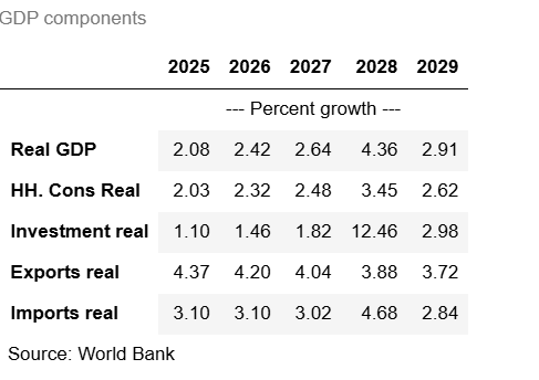
tab.show

GDP components
                         2025   2026   2027   2028   2029
                              --- Percent growth ---     
Real GDP                 2.08   2.42   2.64   4.36   2.91
HH. Cons Real            2.03   2.32   2.48   3.45   2.62
Investment real          1.10   1.46   1.82  12.46   2.98
Exports real             4.37   4.20   4.04   3.88   3.72
Imports real             3.10   3.10   3.02   4.68   2.84
Source: World Bank 

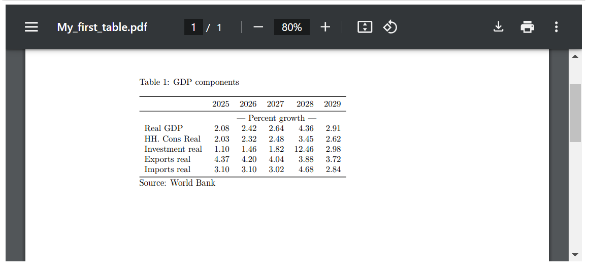
7.2.2.4. The .pdf method causes the table to be rendered to a pdf using latex.

In Jupyter Notebook the rendered file will be displayed within the Jupyter Noteook. Alternatively if the .pdf method is called with the option (pdfopen=True) then the pdf will be opened in a separate browser. In either case, if the table is too large to appear on the pdf page, the scrollbar of the pdf viewer can be used to view the extra columns or rows.

tab.pdf()

Warning

PDF functionality does not work in Google Colab out of the box. Google Colab does not include an installation of latex by default. As a result, when running the PDF routines on Colab they will not render.

Box 10. PDFs and latex outputs

PDF files are generated using Latex as an intermediary. As a result, Latex must be installed on the machine for this option to work. For this publication the Miktex package has been used, and routines have also been tested with the Tex Live package. More on installing the Miktex package can be found here: https://miktex.org/download. When installing Miktex allow automatic download of latex packages.

On a Mac, MacTex can be used. It can be found here: https://www.tug.org/mactex/mactex-download.html

ModelFlow writes the intermediate latex commands from which the pdf is generated to a sub-directory entitled latex one level below the current work directory. The filename will be set to the table_name parameter specified when the table object was declared. Thus, the table called “myTable” will be saved to latex/myTable/MyTable.pdf. The intermediate latex source code is placed in latex/myTable/myTable.tex.

In case of errors or if the user want to enhance the output this file can be edited manually and the pdf re-generated manually using TexWorks which is part of the Miktex instalation.

7.2.3. Table options

7.2.3.1. Data transformations - Growth Rates, Levels, etc.

When the table object is invoked, it defaults to displaying the growth rates for specified variables. However, the constructor supports a range of transformations. Which specification is used is determined by the datatype argument, which can take the following values:

Table: Data Types and Their Meanings

datatype	Meaning
growth	This is the default setting. Growth rate in percent in the most recent dataset (.lastdf).
level	Values in .lastdf.
gdppct	Percentage of GDP in .lastdf.
qoq_ar	Quarterly growth annualized. - Quarterly models only.
Difference views
difgrowth	Change (\(\Delta\)) in growth rates (.lastdf less basedf).
diflevel	Change (\(\Delta\)) in values (.lastdf less basedf).
difgdppct	Change (\(\Delta\)) in the percentage of GDP from (.lastdf less basedf).
difqoq_ar	change in the annualized quarterly growth (.lastdf less basedf)
difpctlevel	Percentage change (\(\Delta\)) in values (.lastdf less basedf).
Values from .basedf
basegrowth	Growth rate in percent in .basedf.
baselevel	Level of the data in .basedf
basegdppct	Percentage of GDP in .basedf.
baseqoq_ar	Quarterly growth in .basedf

7.2.3.2. transpose option

When set, transpose=True (default is False), the table will be rendered so that series appear as columns (with dates progressing downward on the page). In this mode, many time-periods can be displayed, but the number of series will be limited by the width of the paper/screen.

with mpak.set_smpl(2022,2027):
    tab_t = mpak.table(name='A_transposed_table',pat=pat,title='GDP components',
                       foot='Source: World Bank ',transpose = True)
tab_t.show

GDP components
     Real GDP HH. Cons Real Investment real Exports real Imports real
                          --- Percent growth ---                     
2022     0.66          0.80            0.70         4.71         3.00
2023     1.04          1.09            0.63         4.66         2.86
2024     1.60          1.60            0.79         4.53         2.99
2025     2.08          2.03            1.10         4.37         3.10
2026     2.42          2.32            1.46         4.20         3.10
2027     2.64          2.48            1.82         4.04         3.02
Source: World Bank 

7.2.3.3. The dec=## option: limits the decimals displayed

In the example below, only one decimal of the generated table is displayed. Note this table uses the datatype option "pctgdp". which displays the results as a percent of GDP.

Warning

The option datatype='gdppct' is only well-defined for variables that follow World Bank naming conventions and end either (CD,CN, KD or KN). The gdppct routine uses these endings to determine whether to calculate the percent of GDP as a percent of nominal GDP either in local currency (CN) or USD (CD) or real GDP in local currency (KN) or real USD (KD).

pat_gov = '*GGBALOVRLCN *GGDBTTOTLCN *BNCABFUNDCD'
tab_gov = mpak.table(pat_gov,datatype='gdppct',title='In percent of GDP ',dec=1)
tab_gov.show

In percent of GDP 
                                              2025   2026   2027   2028   2029
                                                   --- Percent of GDP ---     
General Government Revenue, Deficit, LCU mn   -3.0   -3.0   -2.9   -2.8   -2.8
General government gross debt millions lcu    57.0   57.3   57.7   57.1   57.5
Current Account Balance, US$ mn               -3.6   -3.5   -3.4   -3.5   -3.4

7.2.4. Handling Table Overruns (too much data)

It is possible to specify a table that is too large for conventional display systems. For example, a table of data taken from a model that covers 100 years could, if the dates run vertically, span more than 1 page, or one that covers many data series might overrun the right hand side of a computer screen, pdf file or printed page. Displaying such tables in Jupyter Notebooks or other computer-based displays is straightforward because Jupyter Notebook will allow the user to scroll content that does not fit on the page. However, in LaTeX documents or printed materials, tables that overrun the page can become impossible to read.

To address this issue, several strategies can be employed:

• Drop Middle Columns: This involves removing several columns from the middle of the table that may not be critical to the reader’s understanding, helping to condense the table into a more manageable size.

• Display Tables in Chunks: Specify a rule for breaking the table into multiple smaller tables, each covering a shorter time span. This not only makes each segment easier to fit on a page but also can help readers digest the information in smaller, more focused increments.

• Display a Slice of Data: Rather than showing the entire timeline, you can display a specific segment or ‘slice’ of the data that is most relevant to the analysis at hand. This approach focuses the reader’s attention and avoids overwhelming them with too much information at once.

These methods can significantly enhance the readability and presentation of large tables when rendered on media that are less flexible than interactive digital platforms.

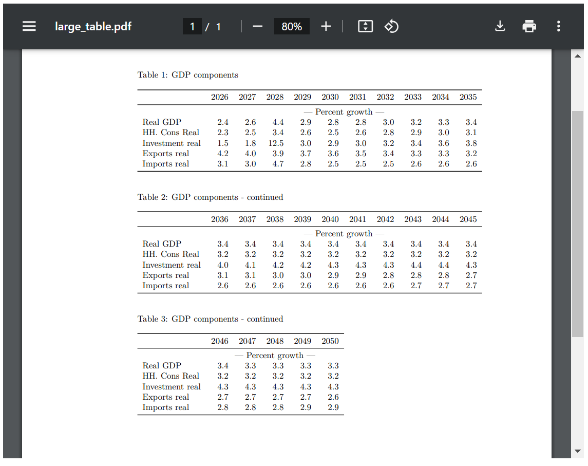
7.2.4.1. Default behavior for dealing with large tables

Below a long table is generated, which runs beyond the edges of the monitor on most computer displays. In Jupyter Notebook or other IDEs elements the standard display options [table name or display(tablename) – both of which produce html ] will generate outputs that that cannot render within one screen width but can scrolled to.

with mpak.set_smpl(2026,2050): 
    tab_large = mpak.table(pat,title='GDP components',name='large_table',dec=1)

display(tab_large)

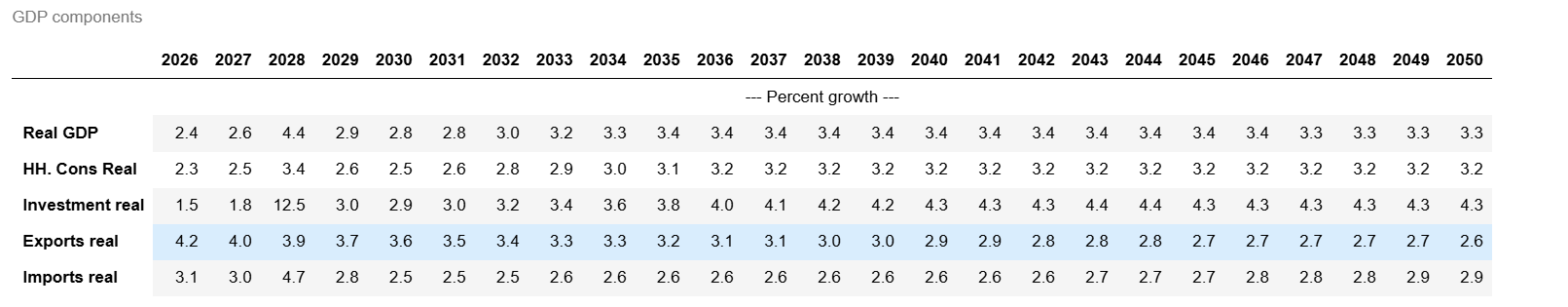
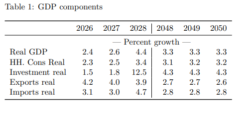
The .show and .pdf methods automatically truncates the width of the table to fit on screen. By default it will show the beginning and ending data columns leaving out the intermediate columns.

tab_large.show

GDP components
                         2026   2027   2028  ...   2048   2049   2050
                                    --- Percent growth ---           
Real GDP                  2.4    2.6    4.4  ...    3.3    3.3    3.3
HH. Cons Real             2.3    2.5    3.4  ...    3.2    3.2    3.2
Investment real           1.5    1.8   12.5  ...    4.3    4.3    4.3
Exports real              4.2    4.0    3.9  ...    2.7    2.7    2.6
Imports real              3.1    3.0    4.7  ...    2.8    2.9    2.9

tab_large.pdf() 

7.2.4.2. Customizing the display of “too large” tables

These default behaviors can be modified using various .table options (see table), notably the options (chunk_size=, time-slice=, tranpose=, max_cols=, last_cols-=) which determine how excess data is treated.

7.2.4.2.1. chunk_size= to split pdf tables.

If the option chunk_size is set. The pdf table will be split into sub tables each with chunk_size columns (except, perhaps, the final table).

tab_large.set_options(chunk_size=10).pdf(height = '700px') 

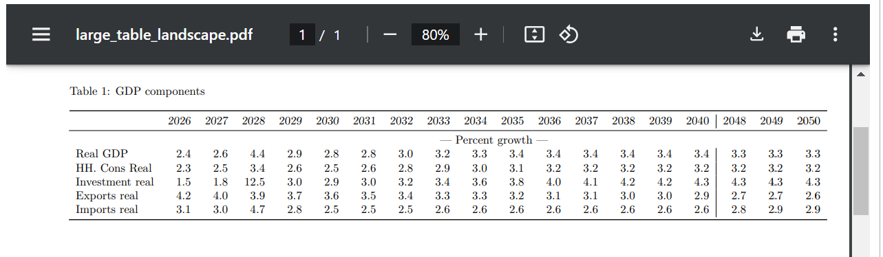
7.2.4.2.2. landscape= to show a pdf in landscape mode. .

If the option landscape= is set. The pdf table will be shown in landscape mode. In this case the max_cols option should also be used, as the default will only be 6.

tab_large.set_options(landscape=True, max_cols=18,name='large_table_landscape').pdf() 

7.2.4.2.3. The timeslice = option allows the user to select which years to render

The timeslice option gives the user full control over which columns (years or quarters) will be displayed displayed.

Beware, timeslice doesn’t care if years are out of order.

In the example below the years are out of order, and the resulting output reflects what was asked for.

tab_large.set_options(timeslice=[2026,2040,2028 ,2029,2050]).show

GDP components
                         2026   2040   2028   2029   2050
                              --- Percent growth ---     
Real GDP                  2.4    3.4    4.4    2.9    3.3
HH. Cons Real             2.3    3.2    3.4    2.6    3.2
Investment real           1.5    4.3   12.5    3.0    4.3
Exports real              4.2    2.9    3.9    3.7    2.6
Imports real              3.1    2.6    4.7    2.8    2.9

In this example, a new table is generated with more conventional timeslices.

with mpak.set_smpl(2026,2050): 
    tab2 = mpak.table(pat,title='GDP components',name='long_table_2',timeslice=[2026,2030,2035 ,2040, 2045, 2050]);
    
tab2.show

GDP components
                         2026   2030   2035   2040   2045   2050
                                  --- Percent growth ---        
Real GDP                 2.42   2.75   3.37   3.41   3.36   3.33
HH. Cons Real            2.32   2.46   3.12   3.17   3.18   3.20
Investment real          1.46   2.92   3.80   4.29   4.34   4.25
Exports real             4.20   3.59   3.19   2.93   2.75   2.64
Imports real             3.10   2.51   2.59   2.58   2.72   2.88

7.2.5. Other ´.table´ options

The table object has two kinds of options:

1. so-called line options that can only be set when the basic table is created with the .table() call.

2. so-called table options can be reset using the set_options method.

Line Options These options are set on table creation.

Argument	Default Value	Description
pat	‘#Headline’ (defined in the ModelFlow class)	variable names to be displayed, may include wildcard specifications
datatype	‘growth’	Defines the data transformation displays (cf. next table)
mul	1.0	Multiplier of values before display
dec	2	set the decimal places to display
col_desc	as shown below	A centered Description of columns (non transposed table)
heading	‘’	A centered text above columns (non transposed table)
rename	True	If True use descriptions else variable names

Table Options These options can be revised after a table has been generated.

Argument	Default Value	Description
name	‘’	Name for this display.
custom_description	{}	Custom description, override default descriptions.
title	‘’	Title.
foot	‘’	Footer.
transpose	False	If True, transposes the table
chunk_size	0	Specifies the number of columns per chunk in tables.
timeslice	[]	Specifies the time slice for data display.
max_cols	6	Maximum columns when displayed as string.
last_cols	3	In Latex, the number of last columns in a display slice.
smpl	(‘’,’’)	set or re-set the smpl for the table

7.2.5.1. Some table examples

Displaying data as the difference in levels. The datatype=diflevel option causes the difference between the level of the selected variables in the .lastdf and .basedf databases to be displayed.

mpak.table(pat,datatype = 'diflevel').show

Table
                        2025   2026   2027        2028        2029
                                  --- Impact, Level ---           
Real GDP                0.01   0.01   0.01  462,356.71  474,302.09
HH. Cons Real           0.00   0.01   0.01  227,277.15  214,784.60
Investment real         0.00   0.01   0.01  336,198.25  361,924.14
Exports real           -0.00  -0.00  -0.00     -530.52   -2,078.90
Imports real            0.00   0.01   0.01  139,487.97  148,662.16

7.2.5.2. The col_desc option causes the default descriptions of variables to be overwritten

The user may change these default descriptors using by setting the col_desc option directly. In the example below, the default text displayed in the previous table is revised to something that is more accurate for this particular example.

mpak.table(pat,datatype = 'diflevel',
           col_desc     = 'Delta, LCU, base year 2000'
        ).show

Table
                                     2025   2026   2027        2028        2029
                                         --- Delta, LCU, base year 2000 ---    
Real GDP                             0.01   0.01   0.01  462,356.71  474,302.09
HH. Cons Real                        0.00   0.01   0.01  227,277.15  214,784.60
Investment real                      0.00   0.01   0.01  336,198.25  361,924.14
Exports real                        -0.00  -0.00  -0.00     -530.52   -2,078.90
Imports real                         0.00   0.01   0.01  139,487.97  148,662.16

If no description is requires set col_desc=' ' That is a single blank.

mpak.table(pat,datatype = 'diflevel',
           col_desc     = ' '
                                   ).show

Table
                  2025   2026   2027        2028        2029
Real GDP          0.01   0.01   0.01  462,356.71  474,302.09
HH. Cons Real     0.00   0.01   0.01  227,277.15  214,784.60
Investment real   0.00   0.01   0.01  336,198.25  361,924.14
Exports real     -0.00  -0.00  -0.00     -530.52   -2,078.90
Imports real      0.00   0.01   0.01  139,487.97  148,662.16

7.3. Complex tables

In the real world more complex tables are often called for, either including a mixture of data display type (some series in levels, others as a percent of GDP) or ones that mix data and text in ways the simple table object does not deal with easily.

A simple solution is to produce and then join two tables, which can be done with the | operator. More complex solutions would involve the report object which allows different table, text and plot elements to be joined in a single report (see the discussion at the end of this chapter).

7.3.1. The | operator joins non-transposed tables

The | operator allows two or more table objects (vertical not transposed) to be combined.

This allows one table expressed in levels (or growth rates) to be combined with another table of data expressed as a percent of GDP. The more complex conjoined table can therefore mix a number of different data representations.

When constructing more complex tables, the heading parameter (heading=some text) can be used to delineate different sections within the combined table. NB: The option heading is case sensitive, Heading= will do nothing.

Note

Non-transposed tables can be joined with transposed tables and figures using the reports functionality described at the end of this chapter.

Below a simple table with a header.

test=mpak.table(heading=r'A test header',pat="PAKNYGDPMKTPKN PAKNYGDPPOTLKN")
test.show

Table
                                 2025   2026   2027   2028   2029
                                          A test header          
                                      --- Percent growth ---     
Real GDP                         2.08   2.42   2.64   4.36   2.91
Potential Output, constant LCU   2.83   2.86   2.88   2.94   3.03

In this example, a more complex table is created as a combination of the earlier generated tables tab and tab_gov, each using different display types.

(tab | tab_gov).show

In percent of GDP 
                                              2025   2026   2027   2028   2029
                                                   --- Percent growth ---     
Real GDP                                      2.08   2.42   2.64   4.36   2.91
HH. Cons Real                                 2.03   2.32   2.48   3.45   2.62
Investment real                               1.10   1.46   1.82  12.46   2.98
Exports real                                  4.37   4.20   4.04   3.88   3.72
Imports real                                  3.10   3.10   3.02   4.68   2.84
                                                   --- Percent of GDP ---     
General Government Revenue, Deficit, LCU mn   -3.0   -3.0   -2.9   -2.8   -2.8
General government gross debt millions lcu    57.0   57.3   57.7   57.1   57.5
Current Account Balance, US$ mn               -3.6   -3.5   -3.4   -3.5   -3.4
Source: World Bank 

Below several different tables are joined to create quite a complex table.

tab_total below is generated as the of several sub tables and illustrates the use of the heading command and the display in a single object of a relatively complex table.

pat=  '*NYGDPMKTPKN *NECONPRVTKN  *NEGDIFTOTKN *NEEXPGNFSKN *NEIMPGNFSKN'
pat_gov = '*GGBALOVRLCN *GGDBTTOTLCN *BNCABFUNDCD'

tab_na_base  = mpak.table(pat,    datatype='basegrowth',
                        heading=r'Baseline')
tab_gov_base = mpak.table(pat_gov,datatype='basegdppct')

tab_na       = mpak.table(pat,    datatype='growth',
                        heading=r'Alternative')
tab_gov      = mpak.table(pat_gov,datatype='gdppct')

tab_na_dif   = mpak.table(pat     ,datatype='difgrowth',
                        heading=r'Impact')
tab_gov_dif  = mpak.table(pat_gov ,datatype='difgdppct') 

# Use the | to concatenate the tabels
tab_total = tab_na_base | tab_gov_base |  tab_na | tab_gov | tab_na_dif | tab_gov_dif

tab_total.show

Table
                                              2025   2026   2027   2028   2029
                                                          Baseline            
                                              --- Baseline Percent growth --- 
Real GDP                                      2.08   2.42   2.64   2.79   2.91
HH. Cons Real                                 2.03   2.32   2.48   2.59   2.69
Investment real                               1.10   1.46   1.82   2.17   2.51
Exports real                                  4.37   4.20   4.04   3.90   3.77
Imports real                                  3.10   3.10   3.02   2.89   2.78
                                              --- Baseline Percent of GDP --- 
General Government Revenue, Deficit, LCU mn  -3.05  -2.98  -2.95  -2.92  -2.91
General government gross debt millions lcu   57.02  57.26  57.69  58.26  58.94
Current Account Balance, US$ mn              -3.55  -3.46  -3.40  -3.37  -3.36
                                                        Alternative           
                                                   --- Percent growth ---     
Real GDP                                      2.08   2.42   2.64   4.36   2.91
HH. Cons Real                                 2.03   2.32   2.48   3.45   2.62
Investment real                               1.10   1.46   1.82  12.46   2.98
Exports real                                  4.37   4.20   4.04   3.88   3.72
Imports real                                  3.10   3.10   3.02   4.68   2.84
                                                   --- Percent of GDP ---     
General Government Revenue, Deficit, LCU mn  -3.05  -2.98  -2.95  -2.81  -2.84
General government gross debt millions lcu   57.02  57.26  57.69  57.11  57.55
Current Account Balance, US$ mn              -3.55  -3.46  -3.40  -3.48  -3.43
                                                           Impact             
                                               --- Impact, Percent growth --- 
Real GDP                                      0.00   0.00   0.00   1.57  -0.00
HH. Cons Real                                 0.00   0.00   0.00   0.86  -0.07
Investment real                               0.00   0.00   0.00  10.29   0.47
Exports real                                 -0.00  -0.00  -0.00  -0.02  -0.05
Imports real                                  0.00   0.00   0.00   1.79   0.06
                                               --- Impact, Percent of GDP --- 
General Government Revenue, Deficit, LCU mn   0.00   0.00   0.00   0.11   0.07
General government gross debt millions lcu   -0.00  -0.00  -0.00  -1.15  -1.39
Current Account Balance, US$ mn               0.00  -0.00  -0.00  -0.11  -0.06

Below the rendering of the same table is revised by using the set_options(smpl=(2025,2026)) modifier on the command line.

# 
tab_total.set_options(smpl=(2026,2030)).show

Table
                                              2026   2027   2028   2029   2030
                                                          Baseline            
                                              --- Baseline Percent growth --- 
Real GDP                                      2.42   2.64   2.79   2.91   3.03
HH. Cons Real                                 2.32   2.48   2.59   2.69   2.78
Investment real                               1.46   1.82   2.17   2.51   2.84
Exports real                                  4.20   4.04   3.90   3.77   3.65
Imports real                                  3.10   3.02   2.89   2.78   2.69
                                              --- Baseline Percent of GDP --- 
General Government Revenue, Deficit, LCU mn  -2.98  -2.95  -2.92  -2.91  -2.90
General government gross debt millions lcu   57.26  57.69  58.26  58.94  59.69
Current Account Balance, US$ mn              -3.46  -3.40  -3.37  -3.36  -3.37
                                                        Alternative           
                                                   --- Percent growth ---     
Real GDP                                      2.42   2.64   4.36   2.91   2.75
HH. Cons Real                                 2.32   2.48   3.45   2.62   2.46
Investment real                               1.46   1.82  12.46   2.98   2.92
Exports real                                  4.20   4.04   3.88   3.72   3.59
Imports real                                  3.10   3.02   4.68   2.84   2.51
                                                   --- Percent of GDP ---     
General Government Revenue, Deficit, LCU mn  -2.98  -2.95  -2.81  -2.84  -2.85
General government gross debt millions lcu   57.26  57.69  57.11  57.55  58.27
Current Account Balance, US$ mn              -3.46  -3.40  -3.48  -3.43  -3.38
                                                           Impact             
                                               --- Impact, Percent growth --- 
Real GDP                                      0.00   0.00   1.57  -0.00  -0.27
HH. Cons Real                                 0.00   0.00   0.86  -0.07  -0.32
Investment real                               0.00   0.00  10.29   0.47   0.09
Exports real                                 -0.00  -0.00  -0.02  -0.05  -0.06
Imports real                                  0.00   0.00   1.79   0.06  -0.17
                                               --- Impact, Percent of GDP --- 
General Government Revenue, Deficit, LCU mn   0.00   0.00   0.11   0.07   0.04
General government gross debt millions lcu   -0.00  -0.00  -1.15  -1.39  -1.42
Current Account Balance, US$ mn              -0.00  -0.00  -0.11  -0.06  -0.01

7.4. The .plot() class

The .plot() class can be used to display results graphically.

The ModelFlow class .plot extends the standard python charting libraries, making them aware of the ModelFlow databases (including kept DataFrames) and provides functionality to display data and results in ways commonly used by macroeconomic modelers.

The class’s constructor is the .plot method which returns an object of type DisplayVarFigDef.

The constructor for .plot takes four arguments:

1. pattern (pat_plot in the example below) which represents a space delimited string containing the mnemonics of the variables (which must be part of the model object to be charted. As with standard ModelFlow search specifications, either mnemonic names, or descriptions can be specified in wildcard specifications.

2. plot_name an identifier for the plot object, used when storing charts that are part of a plot.

3. title A title that will be displayed with any charts that are generated.

4. scenarios, an optional string concatenating with the | symbol the text names of scenarios to be plotted. If left blank (the default) plot will display data from the .lastdf DataFrame or compare the .lastdf results with the data from the .basedf DataFrame.

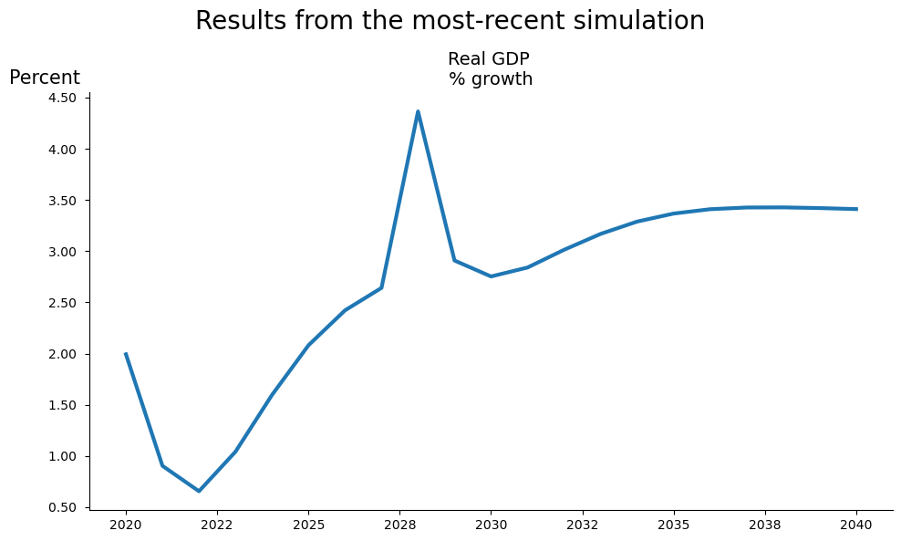
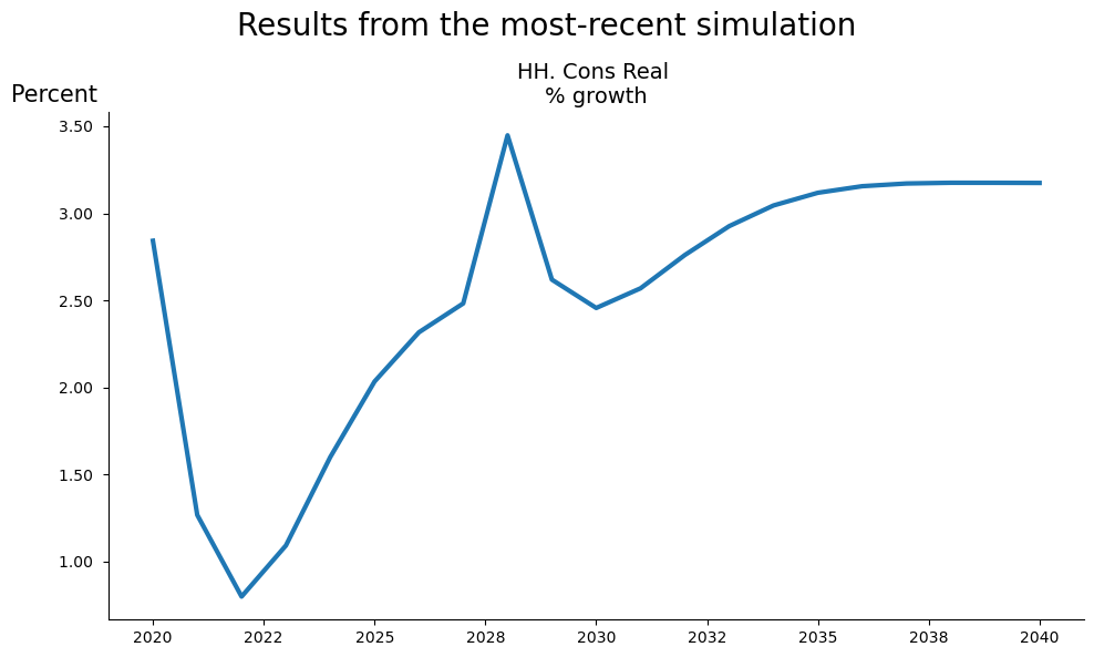
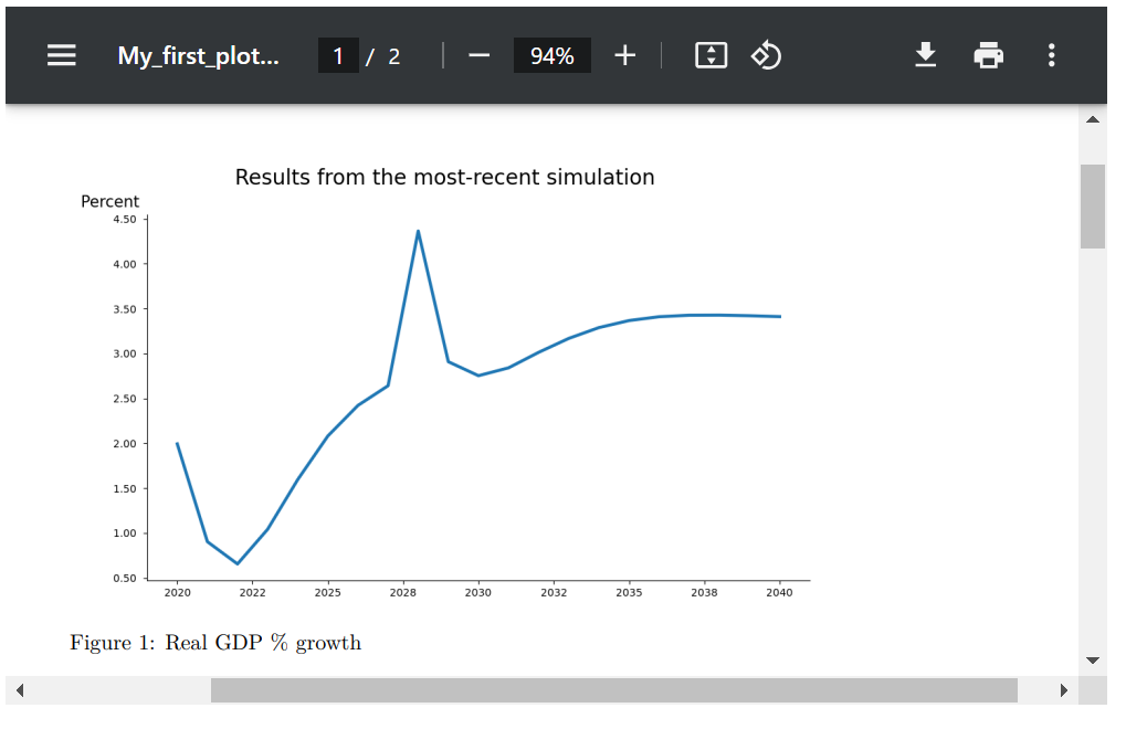
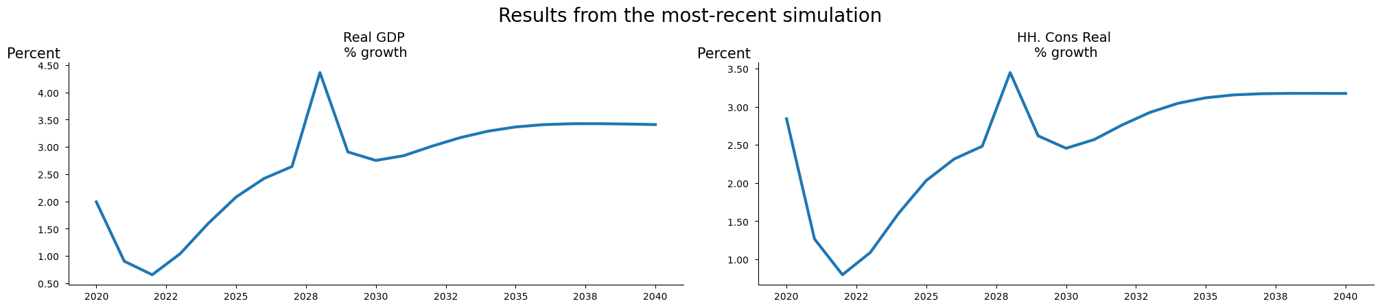
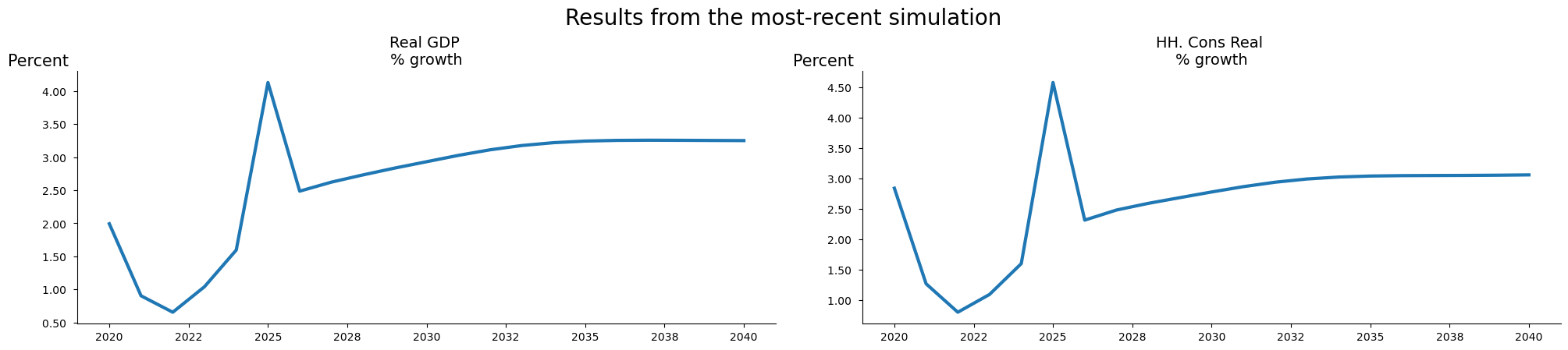
Below the sample period for the model object mpak is set, the pattern that will determine which variables are to be displayed is defined, and a plot object fig is instantiated using the variables in pat_plot, with the name ‘My_first_plot’ and with the displayed title “Results from the most-recent simulation”.

mpak.smpl(2020,2040)
pat_plot=  '*NYGDPMKTPKN *NECONPRVTKN  '
fig = mpak.plot(pat_plot,name='My_first_plot',title="Results from the most-recent simulation")

The object is an instance of the class DisplayVarFigDef. Its construction does not cause the figure to be displayed. Unless the .show method is called explicitly as below.

fig.show;

7.4.1. Rendering a plot object

Like the table object, the plot object has several methods for rendering its figure(s).

These include:

• the name of the object – displays an html widget of the object

• display(object) will display a html widget of the object.

• object.show will show all the charts sequentially

• object.pdf()

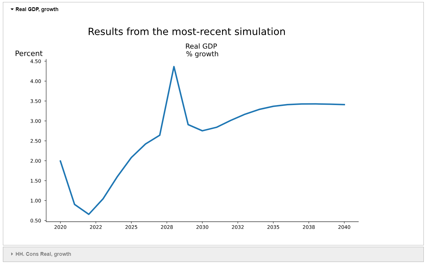
7.4.2. The display (fig) / name of fig command

The first two options: the name of the figure itself executed as a command; and display(nameoffigure) generate exactly the same results.

Under Jupyter Notebook, these two methods generate an “accordion “ widget that allows the user to flip through the various charts (possibly just one) that comprise the plot object.

Different charts in the object can be visualized by selecting the triangle beside the variable name (found on the lefthand side of the screen). Each chart within the plot object has its own triangle beside its name. Selecting one, will fold-up any other figures that may be open and unfold and display the chart associated with the selected variable.

The below command generates the widget comprised of two charts (if more series had been indicated when the figure was instantiated, more widget items would be displayed), one for real GDP growth and the second for real household consumption growth. By default the first is displayed, it can be minimized by clicking on the triangle beside its name. The second (household consumption) will appear under it (below the chart if its is displayed). Click on the triangle beside its name will cause the widget to change the displayed figure to the household consumption chart. Directly clicking on household consumption would have had the same effect, first closing the GDP chart and then displaying the newly selected chart.

display(fig)

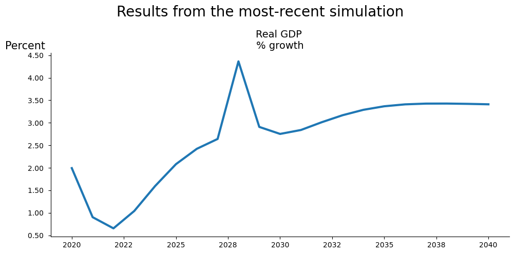
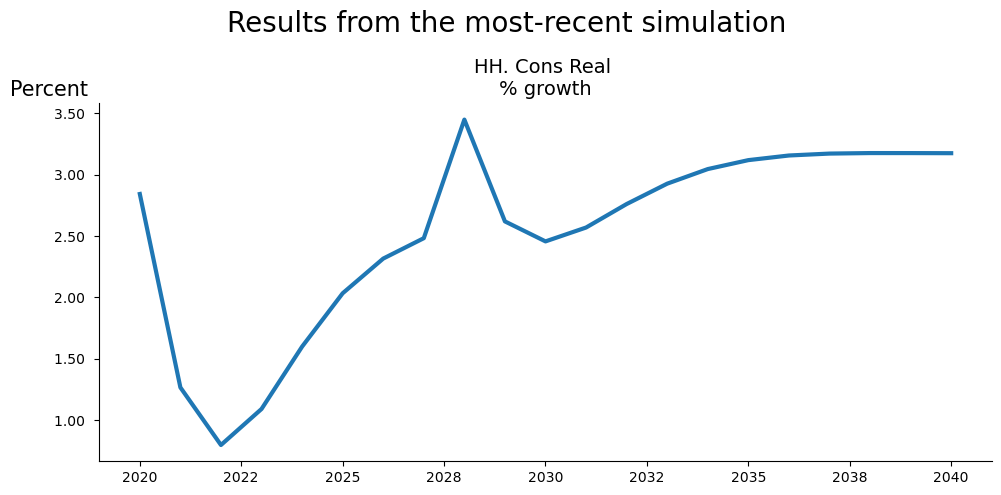
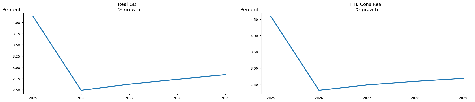
7.4.2.1. The .show method causes each chart in the figure to be displayed sequentially

Here the .set_options() method is used to adjust the display size of the rendered charts.

fig.set_options(size=(10,5)).show

7.4.3. .pdf Creates a .pdf version of the plots

The .pdf method will generate a pdf of the chart(s) that form part of the figure. Each chart will appear sequentially in a single pdf. The generated pdf will be found in a sub-directory with the name that was given to the figure as the root of the pdf file that was generated.

fig.pdf() 

7.4.4. ´.plot´ options

The .plot() object has many options. Like Table these can be split into those that can be set only when the figure is instantiated and those that can be revised later using the .set_options() method. Both types of options are listed below.

Line options are set when the plot is created with the .plot() call and can only be set when the object is instantiated.

Argument	Default Value	Description
pat	‘#Headline’	Pattern with wildcard for variable names
datatype	‘growth’	Defines the datatransformation displayes (cf. next table)
mul	1.0	Multiplier of values before display
ax_title_template	‘’	Template for each chart title

Plot options can be revised after the plot has been created.

Argument	Default Value	Description
rename	True	If True use descriptions else variable names
scenarios	‘’	Show for .basedf/.lastdf or selected scenarios
name	‘’	Name for this display.
custom_description	{}	Custom description, override default descriptions.
title	‘’	Title (used when samefig=True).
samefig	False	If True, displays all chart in the same plot area.
ncol	2	Number of columns when samefig=True.
size	(10, 6)	Specifies the size of each chart
legend	True	If True, includes a legend in the display.
smpl	(‘’,’’)	set smpl for this plot

Like tables, the transformation of the data displayed is controlled by the datatype options, whose parameters are identified below.

7.4.5. Plot Data Types and Scenarios

Tables display output based only on .basedf and .lastdf, the .plot function can also be used to visualize charts based on the scenarios stored in the .keep_solutions dictionary.

• If scenarios='', .plot will display lines corresponding to the data shown in tables, which is based on .basedf and .lastdf.

• If scenarios='<list of scenarios>', .plot will display lines for the data associated with the scenarios specified in the list.

• If scenarios='*', all available scenarios will be plotted.

• If scenarios='base_last', .basedf and .lastdf will be plotted as scenarios.

The table below summarizes how the combination of datatype and scenarios determines the data displayed in the chart.

7.4.5.1. Table: Datatype and Scenario Settings

Datatype	scenarios=’’ or omitted	scenarios=’<list of scenarios>’ (Multiple Scenarios)
Value Views
growth (default)	Growth rate (%) in the most recent dataset (.lastdf).	Growth rates for all scenarios.
level	Values from .lastdf.	Values for all scenarios.
gdppct	Percentage of GDP in .lastdf.	Percentage of GDP for all scenarios.
qoq_ar	Quarterly growth (annualized) for quarterly models in .lastdf.	Quarterly growth (annualized) for all scenarios.
Difference Views
difgrowth	Change (\(\Delta\)) in growth rates between .lastdf and .basedf.	Change (\(\Delta\)) in growth rates between the first and other scenarios.
diflevel	Change (\(\Delta\)) in values between .basedf and .lastdf.	Change (\(\Delta\)) in values between the first and other scenarios.
difgdppct	Change (\(\Delta\)) in the percentage of GDP between .basedf and .lastdf.	Change (\(\Delta\)) in the percentage of GDP between the first and other scenarios.
difqoq_ar	Change in quarterly growth (annualized) between .basedf and .lastdf.	Change (\(\Delta\)) in quarterly growth (annualized) between the first and other scenarios.
difpctlevel	Percentage change (\(\Delta\)) in values between .basedf and .lastdf.	Percentage change (\(\Delta\)) in values between the first and other scenarios.
.basedf Views
basegrowth	Growth rate (%) in .basedf.	Growth rates for the first scenario.
baselevel	Values from .basedf.	Values for the first scenario.
basegdppct	Percentage of GDP in .basedf.	Percentage of GDP for the first scenario.
baseqoq_ar	Quarterly growth (annualized) in .basedf.	Quarterly growth (annualized) for the first scenario.

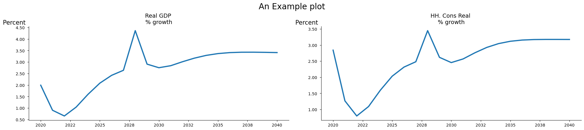
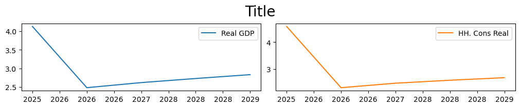
7.4.5.2. The ´samefig=True´ option causes charts to be rendered on a grid

Often a single call to .plot() will result in many charts being produced. The samefig=True option will cause them to be displayed in a grid (rather than the alternative where each chart occupies the full width of the screen or page). This approach both saves real-estate but actually facilitates the comparison of results – across variables, as in the case below; or when used in combination with the by_vars option, across scenarios.

fig.set_options(samefig=True,title='An Example plot').show

7.4.6. The by_var option determines whether to show results by variable (False) or scenario (True)

By default, by_var is set to True and a separate chart is created for each variable in the pat pattern. If multiple scenarios are being inspected, each chart will have a separate line for each scenario.

Setting by_var to False causes plot to generate the charts in the figure by scenario. Each chart shows the value for all specified variables in one scenario, with following charts showing the results for different scenarios.

by_var	a plot for each	a line in each plot for each
True (default)	Variable	Scenario
False	Scenario	Variable

The example below sets both the by_var and samefig options to True. As a result, the charts are displayed in a grid and data for GDP and household consumption (the variables) from one scenario are shown on each graph, with results for one scenario on each graph.

mpak.plot(pat_plot,name='fig_by_scenario',
                       scenarios='Baseline|$25 increase in oil prices 2025-27',
                       datatype='level',samefig=True,
                       by_var=False,legend=False,mul=1/1_000_000).show

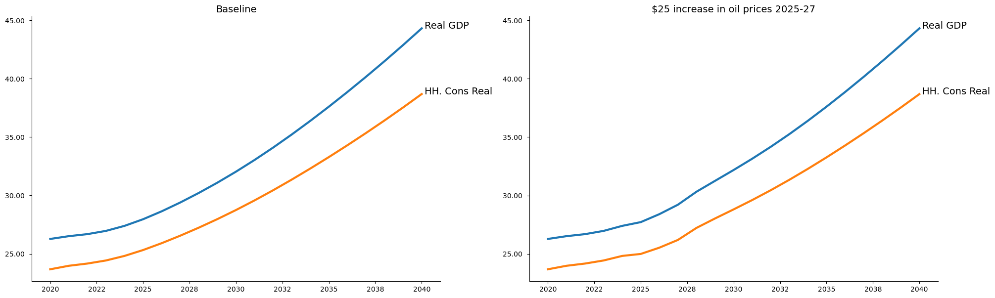
The example also illustrates the use of the legend and mul options. The option legend=False suppresses the legend (as a box with all series description in one place) and instead causes the series labels to be placed to the right of the line of each rendered series.

The mul=1/1_000_000 option causes the axis to be rendered in millions. Notice python allows large numbers to be split by _ which makes them more readable. It is not necessary to do this.

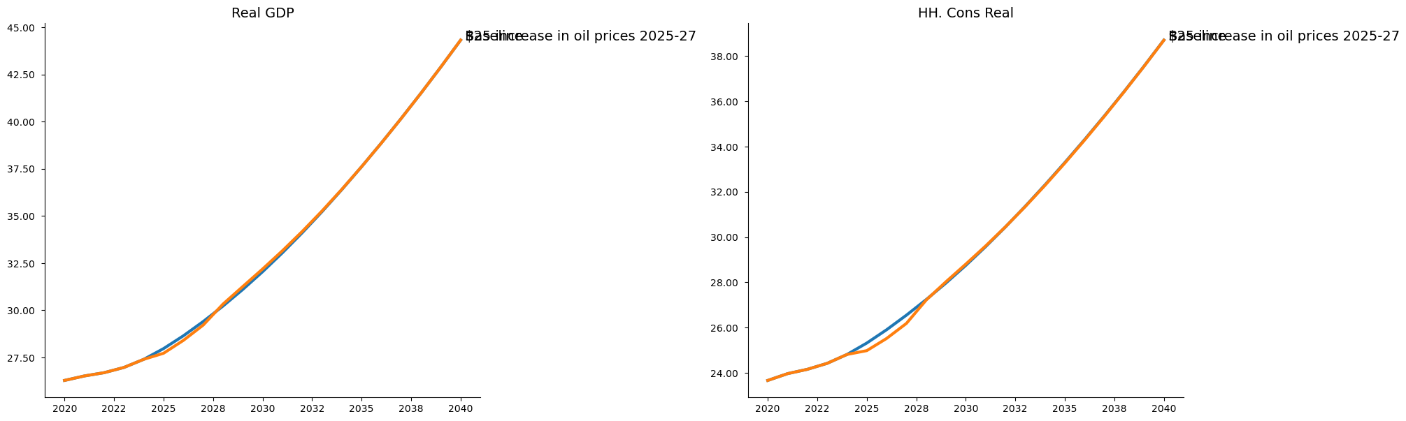
Below the same two results are shown but organized by variable with the by_var option set to True.

mpak.plot(pat_plot,name='fig_by_scenario',
                       scenarios='Baseline|$25 increase in oil prices 2025-27',
                       datatype='level',samefig=True,
                       by_var=True,legend=False,mul=1/1_000_000).show

7.4.7. The scenarios= option selects the scenarios to be displayed

The scenarios= option allows the user to specify which scenarios (from the kept scenarios in the model object) to use in generating the plots. Scenarios names must be the exact match to the text used when the keep command was executed, and must be separated by the | symbol.

Recall

To find all names of the stored scenarios use:

for key  in mpak.keep_solutions:
    print(key);

Baseline
$25 increase in oil prices 2025-27
2.5% increase in C 2025-40
2.5% increase in C 2025-27 -- exog whole period
2.5% increase in C 2025-27 -- exog whole period --KG=True
2.5% increase in C 2025-27 -- temporarily exogenized
1% of GDP increase in FDI and private investment (AF shock)

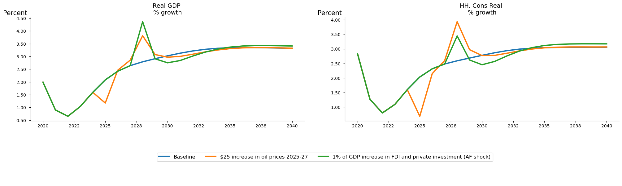
In the example below, the same pattern as before is utilized (real GDP and real household expenditure), but the scenarios option indicates that the charts should be generated from three scenarios:

1. Baseline

2. “$25 increase in oil prices 2025-27”;

3. “1% of GDP increase in FDI and private investment (AF shock)”.

In this use-case the datatype=’growth’ causes the growth rate from each scenario to be rendered.

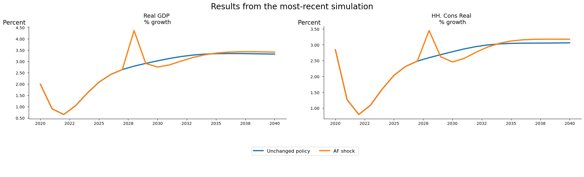
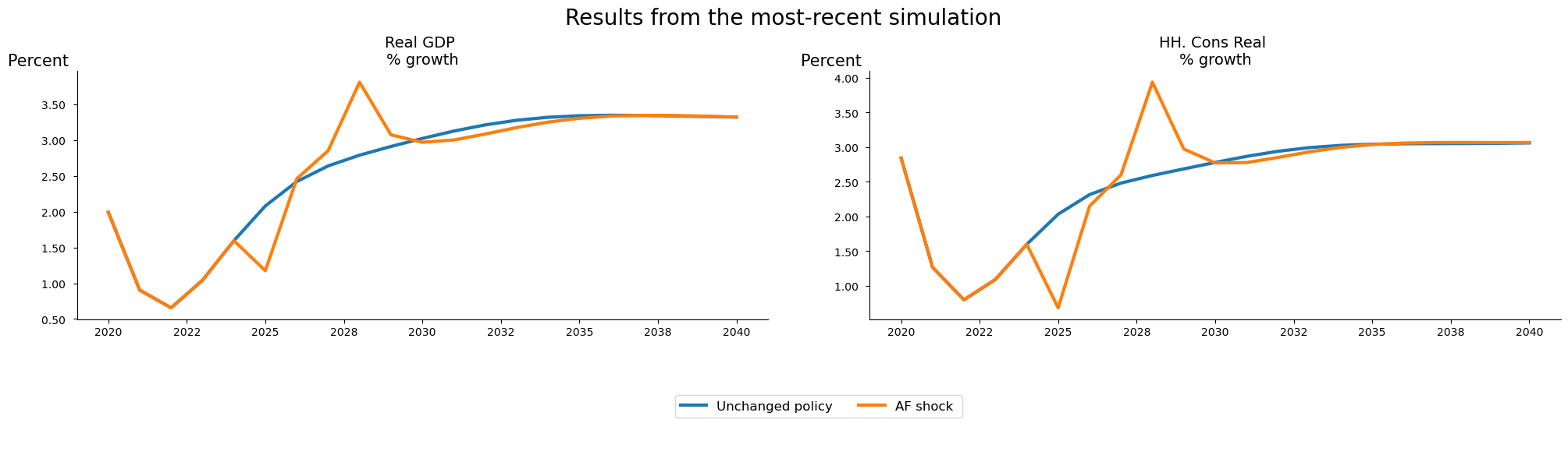
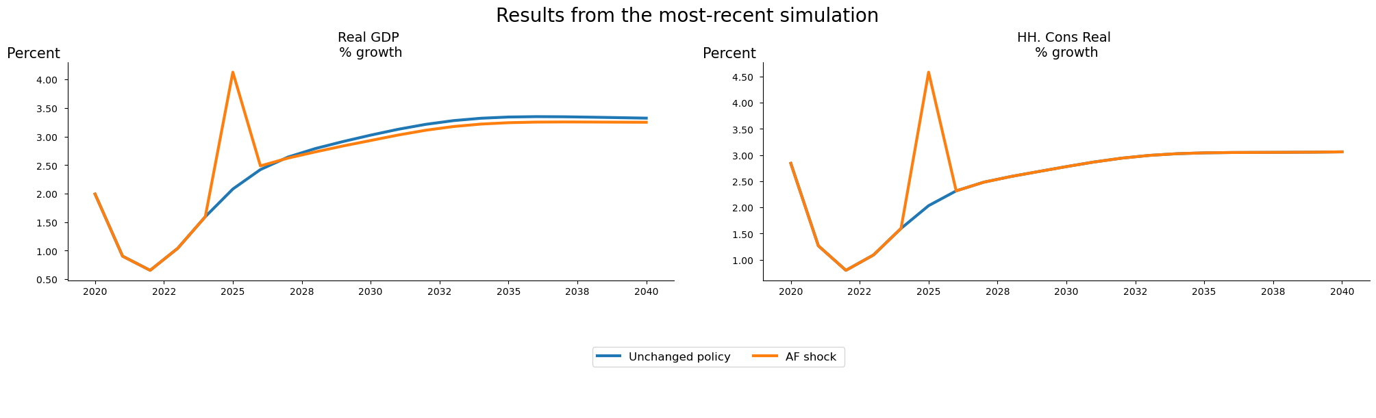
mpak.plot(pat_plot,name='fig_select',datatype='growth',samefig=True,
         scenarios='Baseline|$25 increase in oil prices 2025-27|1% of GDP increase in FDI and private investment (AF shock)').show

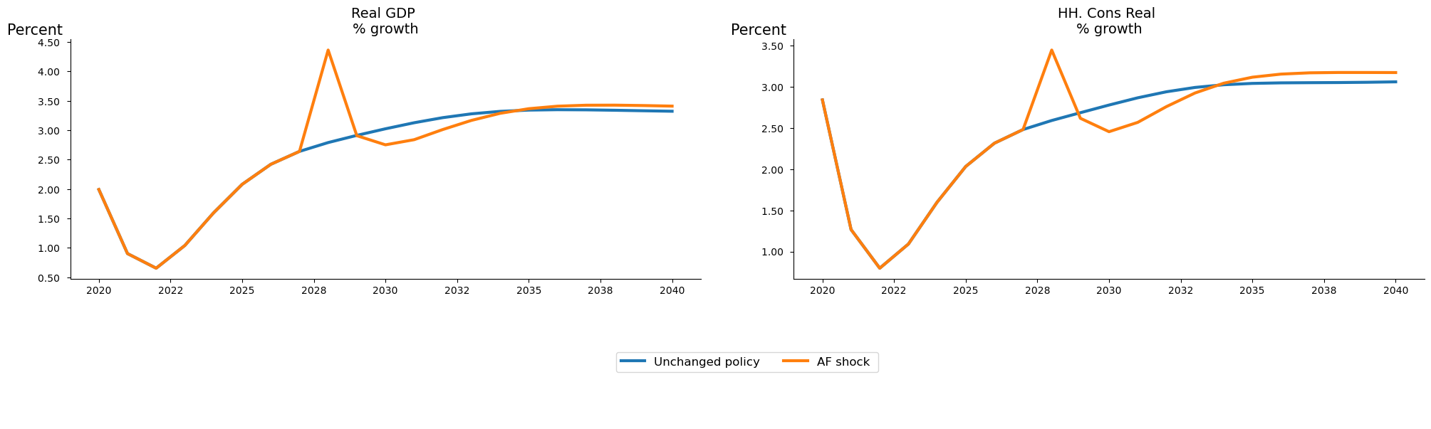
7.4.7.1. The special scenario base_last

The scenario option base_last will use the .basedf and .lastdf as scenarios dataframes as the scenarios.

mpak.plot(pat_plot,name='fig_select',datatype='growth',samefig=True,
         scenarios='base_last').show

7.4.7.1.1. .basename .lastname can be used to rename the scenarios

mpak.basename = 'Unchanged policy'
mpak.lastname = 'AF shock '
mpak.plot(pat_plot,name='fig_select',datatype='growth',samefig=True,
         scenarios='base_last').show

7.4.8. Template for each chart title: ax_title_template

The text associated with each graph can be customized by using the ax_title_template option.

ax_title_template can be sent to any arbitrary string. If the string contains the special characters {var_name}, and/ or {var_description} or {compare} then the name of the variable being displayed (or its description) or the name of the baseline scenario will be substituted for the expression in the figure.

Placeholder	Replaced by
{var_name}	Variable Mnemonic
{var_description}	Variable description
{compare}	First scenario used for comparison

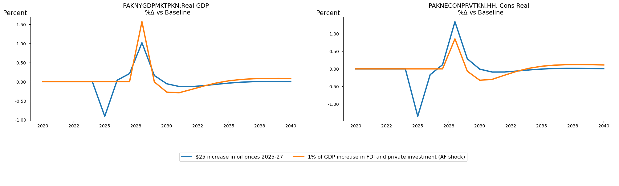
In the example below, all three placeholders are utilized, and the text includes a LaTeX expression (the sub-string $\Delta\$) bordered by $ signs, which renders in the chart as the Greek symbol \(\Delta\).

mpak.plot(pat_plot,datatype='difgrowth',
          scenarios='Baseline|$25 increase in oil prices 2025-27|1% of GDP increase in FDI and private investment (AF shock)',
          samefig=True,
        ax_title_template= r'{var_name}:{var_description} \n %$\Delta$ vs {compare}' ).show

7.4.9. Joing plots with |

Like Tables, Plots can be concatenated together using the | operator. This allows plots with different datatypes to be displayed together.

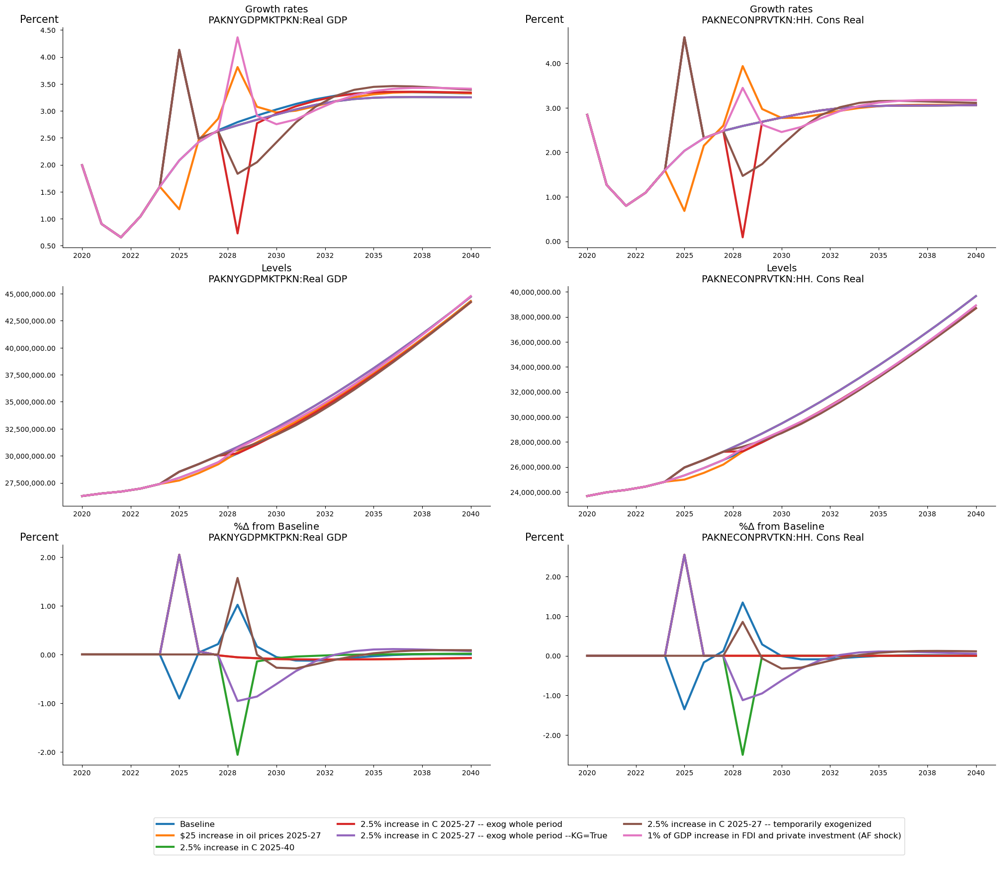
In the example below, results for GDP in each scenario and household consumption for each scenario are displayed first as growth rates, secondly as levels, and finally as changes in the growth rates.

The three separate figures are then joined in the figure called fig_, with the samefig=True flag set so that the six separate charts are arranged in a grid to facilitate reading and comparison.

fig1 = mpak.plot(pat_plot,name='growth',scenarios='*',ax_title_template= r'Growth rates\n {var_name}:{var_description}')
fig2 = mpak.plot(pat_plot,datatype='level',scenarios='*',ax_title_template= r'Levels\n {var_name}:{var_description}')
fig3 = mpak.plot(pat_plot,datatype='difgrowth',name= 'dif',
                 ax_title_template= r'%$\Delta$ from {compare}\n {var_name}:{var_description}',
                 scenarios='*')
fig_ = (fig1 | fig2 | fig3).set_options(samefig=True,name='fig_')
fig_.show

7.4.10. .savefigs() Saving plots in other formats.

Plots are created using the matplotlib library. If charts are going to be used further downstream they can be saved to file using a wide range of formats.

.savefigs() options

Parameter	Type	Description	Default
location	str	The folder in which to save the charts.	'./graph'
experimentname	str	A subfolder under location where charts are saved.	'experiment1'
addname	str	An additional name added to each figure filename.	'' (empty string)
extensions	list	A list of file extensions for saving the figures.	['svg']
xopen	bool	If True, open the saved figure locations in a web browser.

Charts can be saved using the following formats:

Extension	Description
.png	Portable Network Graphics
.jpg or .jpeg	t Photographic Experts Group
.tif or .tiff	Tagged Image File Format
.bmp	Bitmap
.gif	Graphics Interchange Format
.svg	Scalable Vector Graphics
.pdf	Portable Document Format
.eps	Encapsulated PostScript
.ps	PostScript
.raw	Raw image data
.rgba	Raw RGBA bitmap
.pgf	Portable Graphics Format

An example:

fig_for_saving = mpak.plot(pat_plot,name='for_saving')
fig_for_saving.savefigs() 

'Saved at: graph/experiment1'

In this example the sub-directory name where the files will be saved is changed to Scenario1 and two copies of the each chart is saved, once as an SVG file the other as a PDF, by setting the extensions option to a list extensions=['svg','pdf'].

fig_for_saving = mpak.plot(pat_plot,name='for_saving',experimentname="Scenario1");
fig_for_saving.savefigs(extensions=['svg','pdf']) 

'Saved at: graph/experiment1'

7.5. The .text() class

The .text() class is less complex than the .plot() and .table() procedures. It is mainly used implicitly in Reports, but can be declared as an object and used either in a report or on its own.

The text class allows the user to define three different types of text: .text_text .html_text and .latex_text. These properties are optional and can be declared explicitly or implicitly.

object	delimited by	contains
.text_text	nothing	Plain text
.html_text	<html> </html>	html text
.latex_text	<latex> </latex>	latex text

A text object can be declared in the same way as the .plot or table(), called in conjunction with a model object. In the example below we create an object mytext, and implicitly set the .text_text property to “Some text”. The html and latex properties are undeclared.

mytext=mpak.text("Some text")
mytext.show

Some text

In the example below a more complicated object is declared.

Note this is a multiline text object, and that the plain text, html and latex properties are all declared implicitly with the html text demarcated by the <html></html> tokens and the latex text similarly demarcated by the tokens.

multimodeText=mpak.text(r'''
Example of plain output
This is the plain contents of a multiline text 
object.
<html><h1> Example of html output</h1>
This is the <b>html content</b> of a multiline text<b>
object.</b>
</html>
<latex>
\section*{Example of latex output}
This is the \textbf{latex content} of a  multiline text
\textbf{object} 
</latex>
''')

The three different kinds of text that can be included in a text object can be extracted from the text object.

print(multimodeText.text_text)
print(multimodeText.html_text)
print(multimodeText.latex_text)

Example of plain output
This is the plain contents of a multiline text 
object.

<h1> Example of html output</h1>
This is the <b>html content</b> of a multiline text<b>
object.</b>


\section*{Example of latex output}
This is the \textbf{latex content} of a  multiline text
\textbf{object} 

7.5.1. Renderings

When rendered as text, the text object will ignore the html and latex portions. When rendered as html it will ignore the text and latex. The pdf rendering ignores text and html.

Warning

Because the text of the three internal components of the text object (plain text, html and latex} are independent of one another they can hold completely unrelated text. While this might be useful in some contexts, in most, the three formulations should contain the same message even if the embellishments may differ somewhat given the capabilities of the rendering engine.

7.5.2. Html renderings

Executing the text object directly from the command line will cause it to render as html. By the same token, the function Display() when called on a text object will render it as text. NB: if there is no html object, the plain text version will be rendered.

multimodeText

display(multimodeText)

7.5.3. Simple text rendering

The .show method will render the object as plain text.

multimodeText.show

Example of plain output
This is the plain contents of a multiline text 
object.

7.5.4. Pdf rendering

Finally the .pdf() method will r4edner the object’s latex contents rendered to a pdf file.

multimodeText.pdf()

7.6. Reports

Joined tables and plots offer significant flexibility, but have limitations. In particular, joined tables must cover the same time-period, and tables cannot be joined with plots, while transposed tables cannot be joined with other tables.

Reports in ModelFlow are containers that can contains figures, plots, tables of different dimension and text. Moreover, Report objects can be saved in a model object and regenerated on new data without requiring any additional effort by the user.

7.6.1. Creating a report

A report can be generated by combining tables, plots, text and even other reports with the + operator.

Below a small report is generated from two tables generated earlier in this chapter (tab and its transpose tab_t and a the plot object fig.

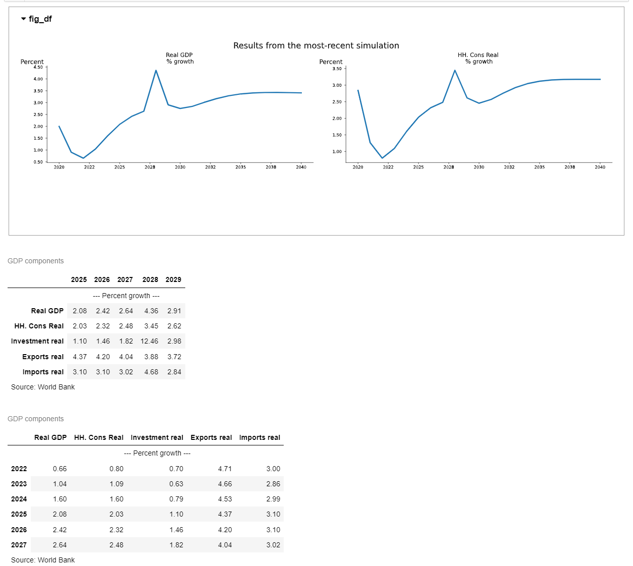
mpak.smpl(2020,2040)
smallreport = (fig.set_options(samefig=True,name='fig_df',scenarios='base_last')+tab+tab_t).set_name('small report')

The code instantiates a new report object called smallreport. The objects included in the report are brought together by the + operator.

These include the previously defined object fig, whose options are adjusted with the fig.set_options(samefig=True) command. This alters the resulting output such that the charts in the original fig are organized in a grid (samefig=True). The Report is completed by adding the previously defined tables: tab with years as columns and, tab_twith years as rows.

The method .set_name('small report') gives the report a name, which identifies the container (and determines where its file outputs will be saved if a pdf version is generated).

Warning

The report name will be used in a dictionary of reports to identify the report. As a result, users should ensure that each report has a unique name.

7.6.2. Rendering a report

Reports can be displayed using the same mechanisms as tables and plot. Either by executing the name of the report itself, or with the command display(reportname), or with reportname.show or reportname.pdf.

Below is the output from the .show method

smallreport.show 

GDP components
                         2025   2026   2027   2028   2029
                              --- Percent growth ---     
Real GDP                 2.08   2.42   2.64   4.36   2.91
HH. Cons Real            2.03   2.32   2.48   3.45   2.62
Investment real          1.10   1.46   1.82  12.46   2.98
Exports real             4.37   4.20   4.04   3.88   3.72
Imports real             3.10   3.10   3.02   4.68   2.84
Source: World Bank 


GDP components
     Real GDP HH. Cons Real Investment real Exports real Imports real
                          --- Percent growth ---                     
2022     0.66          0.80            0.70         4.71         3.00
2023     1.04          1.09            0.63         4.66         2.86
2024     1.60          1.60            0.79         4.53         2.99
2025     2.08          2.03            1.10         4.37         3.10
2026     2.42          2.32            1.46         4.20         3.10
2027     2.64          2.48            1.82         4.04         3.02
Source: World Bank 

The reportname alone or display(report) will render the report as html (suitable for Jupyter Notebooks or a computer screen. The figure is rendered as an interactive widget the same as a normal figure.

display(smallreport)

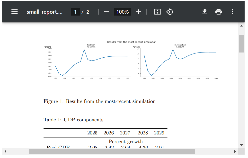
The PDF rendering will show each chart separately (like the .show command) or if the samefig=True option is selected (as is the case here) the charts will be organized in a grid.

smallreport.pdf()

7.6.3. A report with different text

Unlike a table or a plot, a report can be customized by adding unlimited amounts of text.

In the example below text is entered using three formats – plain text, Latex, and html.

Doing so in this way allows each rendering engine to do its best.

If separate text is not entered between the <html> and </html> tags or between <latex></latex> tags then the html and pdf outputs will use the plain text inputs.

If the text under html or latex tags differs from the plain text, the latex text will be used for pdfs and the html for html outputs.

Below the same content as in the small report but with annotated with text.

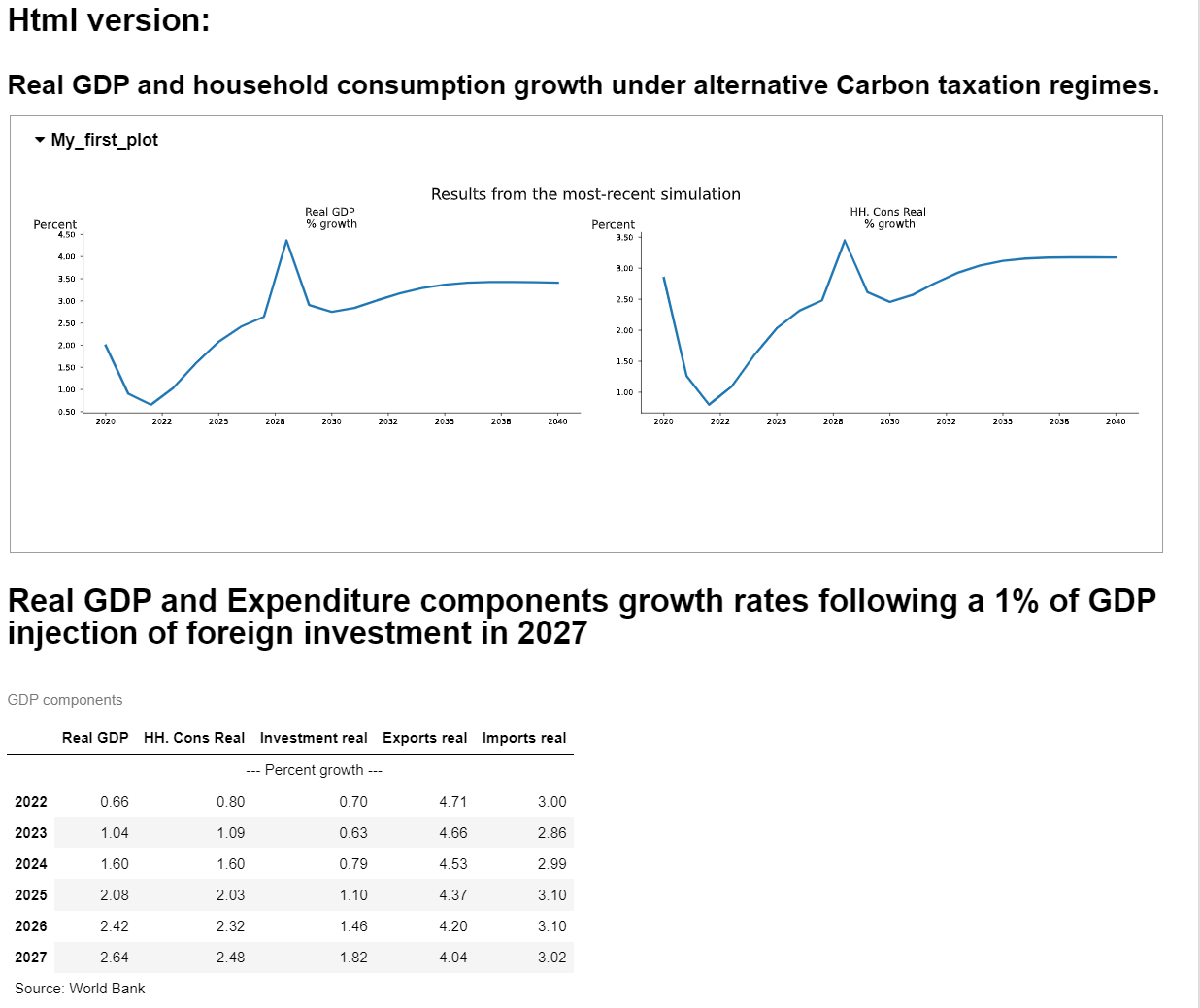
textreport=(r'''
Text version: Real GDP and household consumption growth under alternative Carbon taxation regimes.
<latex>
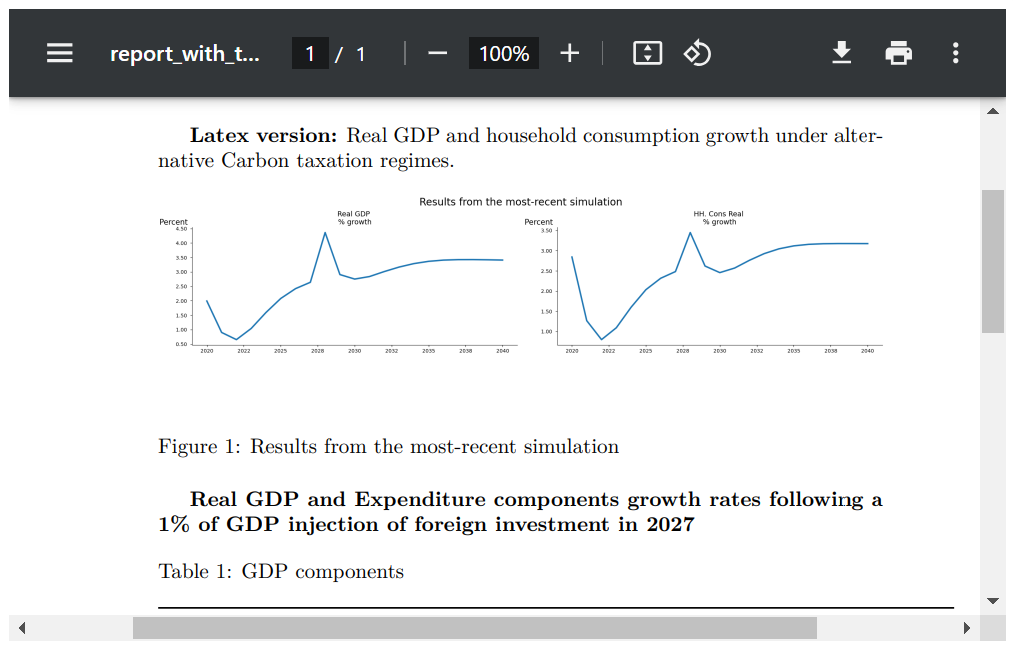
\textbf{Latex version:} Real GDP and household consumption growth under alternative Carbon taxation regimes.
</latex>
<html>
<h1>Html version:</h1>
<h2> Real GDP and household consumption growth under alternative Carbon taxation regimes.</h2>
</html>
''' + 
fig.set_options(samefig=True)+
r'''Real GDP and Expenditure components growth rates following a 1% of GDP injection of foreign investment in 2027
<latex>
\textbf{Real GDP and Expenditure components growth rates following a 1\% of GDP injection of foreign investment in 2027}
</latex>
<html>
<h1>Real GDP and Expenditure components growth rates following a 1% of GDP injection of foreign investment in 2027</h1>
</html>''' +        
tab_t).set_name('report_with_text')

When rendered as text, no special formatting of the text is done.

textreport.show   

Text version: Real GDP and household consumption growth under alternative Carbon taxation regimes.

Real GDP and Expenditure components growth rates following a 1% of GDP injection of foreign investment in 2027



GDP components
     Real GDP HH. Cons Real Investment real Exports real Imports real
                          --- Percent growth ---                     
2022     0.66          0.80            0.70         4.71         3.00
2023     1.04          1.09            0.63         4.66         2.86
2024     1.60          1.60            0.79         4.53         2.99
2025     2.08          2.03            1.10         4.37         3.10
2026     2.42          2.32            1.46         4.20         3.10
2027     2.64          2.48            1.82         4.04         3.02
Source: World Bank 

When rendered as html, the html text is used and html formatting is rendered.

textreport

Finally when rendered as a pdf, the pdf specific text and formatting is used.

textreport.pdf()   

7.7. Storing .reports definitions for later use

The definitions of the different reports can be stored in the .reports dictionary that is part of the model object so they can be retrieved and used later.

Notice it is the definition not the content of the table which is stored. So when applied later it is the values of the variables of that model object (notably the .lastdf and .basedf dataframes of the model object at that point in time that will be rendered.

The .reports dictionary is saved when the model is dumped with .modeldump and restored when the function model.modelload() is used to load a model.

Note

A table, plot and text objects are each special cases of a report and can be stored as well.

7.7.1. The method .add_report adds a report to the .reports dictionary.

mpak.add_report([tab_large,smallreport,textreport])

Reports added to report repo: large_table, small_report, report_with_text

for key in mpak.reports:
    print(key);

large_table
small_report
report_with_text

7.7.2. The .get_report method creates a report from a stored specification.

A report can be retrieved from the model object and assigned to a variable. Changes to that new report will not be stored unless explicitly saved.

newreport=mpak.get_report('small_report').show  

GDP components
                         2025   2026   2027   2028   2029
                              --- Percent growth ---     
Real GDP                 2.08   2.42   2.64   4.36   2.91
HH. Cons Real            2.03   2.32   2.48   3.45   2.62
Investment real          1.10   1.46   1.82  12.46   2.98
Exports real             4.37   4.20   4.04   3.88   3.72
Imports real             3.10   3.10   3.02   4.68   2.84
Source: World Bank 


GDP components
     Real GDP HH. Cons Real Investment real Exports real Imports real
                          --- Percent growth ---                     
2022     0.66          0.80            0.70         4.71         3.00
2023     1.04          1.09            0.63         4.66         2.86
2024     1.60          1.60            0.79         4.53         2.99
2025     2.08          2.03            1.10         4.37         3.10
2026     2.42          2.32            1.46         4.20         3.10
2027     2.64          2.48            1.82         4.04         3.02
Source: World Bank 

7.7.3. Re-using a report on multiple simulation results

In this example the small_report is populated with results from three different simulations and the results displayed (see the above listing for names of scenarios in the kept_scenarios dictionary).

mpak.basedf = mpak.keep_solutions['Baseline']
mpak.lastdf = mpak.keep_solutions['1% of GDP increase in FDI and private investment (AF shock)']
mpak.smpl(2025,2029);


firstreport=mpak.get_report('small_report').set_name('firstreport').show

GDP components
                         2025   2026   2027   2028   2029
                              --- Percent growth ---     
Real GDP                 2.08   2.42   2.64   4.36   2.91
HH. Cons Real            2.03   2.32   2.48   3.45   2.62
Investment real          1.10   1.46   1.82  12.46   2.98
Exports real             4.37   4.20   4.04   3.88   3.72
Imports real             3.10   3.10   3.02   4.68   2.84
Source: World Bank 


GDP components
     Real GDP HH. Cons Real Investment real Exports real Imports real
                          --- Percent growth ---                     
2022     0.66          0.80            0.70         4.71         3.00
2023     1.04          1.09            0.63         4.66         2.86
2024     1.60          1.60            0.79         4.53         2.99
2025     2.08          2.03            1.10         4.37         3.10
2026     2.42          2.32            1.46         4.20         3.10
2027     2.64          2.48            1.82         4.04         3.02
Source: World Bank 

mpak.basedf = mpak.keep_solutions['Baseline']
mpak.lastdf = mpak.keep_solutions['$25 increase in oil prices 2025-27']
mpak.smpl(2025,2029);
secondreport=mpak.get_report('small_report').set_name('secondreport').show  

GDP components
                         2025   2026   2027   2028   2029
                              --- Percent growth ---     
Real GDP                 1.18   2.46   2.85   3.81   3.08
HH. Cons Real            0.68   2.15   2.60   3.94   2.97
Investment real          1.23   0.99   1.62   2.02   2.93
Exports real             4.36   4.21   4.06   3.92   3.78
Imports real             1.57   1.88   2.45   3.98   3.74
Source: World Bank 


GDP components
     Real GDP HH. Cons Real Investment real Exports real Imports real
                          --- Percent growth ---                     
2022     0.66          0.80            0.70         4.71         3.00
2023     1.04          1.09            0.63         4.66         2.86
2024     1.60          1.60            0.79         4.53         2.99
2025     1.18          0.68            1.23         4.36         1.57
2026     2.46          2.15            0.99         4.21         1.88
2027     2.85          2.60            1.62         4.06         2.45
Source: World Bank 

mpak.basedf = mpak.keep_solutions['Baseline']
mpak.lastdf = mpak.keep_solutions['2.5% increase in C 2025-27 -- exog whole period --KG=True']
mpak.smpl(2025,2029);
thirdreport=mpak.get_report('small_report').set_name('thirdreport').show  

GDP components
                         2025   2026   2027   2028   2029
                              --- Percent growth ---     
Real GDP                 4.13   2.49   2.62   2.73   2.84
HH. Cons Real            4.58   2.32   2.48   2.59   2.69
Investment real          2.50   2.12   2.23   2.45   2.69
Exports real             4.35   4.14   3.96   3.80   3.66
Imports real             5.44   3.27   3.18   3.08   2.99
Source: World Bank 


GDP components
     Real GDP HH. Cons Real Investment real Exports real Imports real
                          --- Percent growth ---                     
2022     0.66          0.80            0.70         4.71         3.00
2023     1.04          1.09            0.63         4.66         2.86
2024     1.60          1.60            0.79         4.53         2.99
2025     4.13          4.58            2.50         4.35         5.44
2026     2.49          2.32            2.12         4.14         3.27
2027     2.62          2.48            2.23         3.96         3.18
Source: World Bank 

7.7.4. Reports are stored in .pcim files, and restored when a model is loaded

Once a report has been added to the model object it will be saved with the model object.

Below we save the current state of mpak, inclusive of the reports that were added to the model object. So first dump the model and data:

mpak.modeldump('testpak',keep=True)

Next a new model object is declared tempmodel, and the state and data from the saved mpak are read into that object.

xpak,baseline = model.modelload('testpak',run=True  )

Zipped file read:  testpak.pcim

Next the .basedf and .lastdf dataframes are set equal to the data frames from the kept Baseline and investment shock scenarios.

xpak.basedf = xpak.keep_solutions['Baseline']
xpak.lastdf = xpak.keep_solutions['1% of GDP increase in FDI and private investment (AF shock)']

With that, the reports can be run (and should show precisely the same results).

trep=xpak.get_report('report_with_text')
trep.show

Text version: Real GDP and household consumption growth under alternative Carbon taxation regimes.

Real GDP and Expenditure components growth rates following a 1% of GDP injection of foreign investment in 2027



GDP components
     Real GDP HH. Cons Real Investment real Exports real Imports real
                          --- Percent growth ---                     
2022     0.66          0.80            0.70         4.71         3.00
2023     1.04          1.09            0.63         4.66         2.86
2024     1.60          1.60            0.79         4.53         2.99
2025     4.13          4.58            2.50         4.35         5.44
2026     2.49          2.32            2.12         4.14         3.27
2027     2.62          2.48            2.23         3.96         3.18
Source: World Bank 

7.8. [].rtable and [].rplot - reports from []

Report tables and plots can also be created directly from the variable selector []. The purpose is to enable easy reuse of variable selection like this.

mpak['PAKNYGDPMKTPKN PAKNECONPRVTKN'].growth.rename().plot();

To a plot like this:

mpak['PAKNYGDPMKTPKN PAKNECONPRVTKN'].rplot(samefig=1).show 

Or a table like this:

mpak['PAKNYGDPMKTPKN PAKNECONPRVTKN'].rtable(samefig=1).show 

Table
                         2025   2026   2027   2028   2029
                              --- Percent growth ---     
Real GDP                 4.13   2.49   2.62   2.73   2.84
HH. Cons Real            4.58   2.32   2.48   2.59   2.69

The [].rtable and [].rplot are just wrappers around the model instance.plot and model instance.table so the arguments - except the variable selection - are the same, and the returne values can be used just the returned values of model instance.plot and model instance.table. So + and | can also be used.

(mpak.text('Growth in {cty_name}') + 
mpak['PAKNYGDPMKTPKN PAKNECONPRVTKN'].rplot(samefig=1) + 
mpak['PAKNYGDPMKTPKN PAKNECONPRVTKN'].rtable()).show

Growth in Pakistan

Table
                         2025   2026   2027   2028   2029
                              --- Percent growth ---     
Real GDP                 4.13   2.49   2.62   2.73   2.84
HH. Cons Real            4.58   2.32   2.48   2.59   2.69

7.9. Some other supported outputs

Below are an illustration of some charts and table features not discussed above, which may be of interest in some contexts:

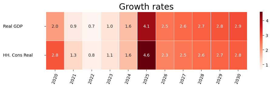
7.9.1. Heatmaps

For some model types heatmaps can be helpful, and they come out of the box.

with mpak.set_smpl(2020,2030):
    mpak['PAKNYGDPMKTPKN PAKNECONPRVTKN'].pct.rename().heat(title='Growth rates',annot=True,dec=1,size=(10,3))