4. Scenario analysis

Building and running scenarios is central to working with a macroeconomic model. Scenarios help to quantify the expected impacts of different policies and external events. In so doing they give valuable insights to policy makers concerning potential policies. This chapter introduces users to scenario analysis using World Bank models and ModelFlow. The scenarios presented are relatively simple, but cover all of the different kind of scenarios typically performed and insights into how to get around shortcomings that a specific model may have for a given question.

In this chapter - Scenario Analysis

This chapter presents examples of running simulations. Four types of simulation are covered:

1. Permanent Exogenous Shocks: These involve either shocking an exogenous variable (say World oil prices) or deactivating an equation and treating its dependent variable as if it were exogenous and shocking it directly.

2. Endogenous Shocks: In these shocks, a behavioral equation is left active, but its add-factor is shocked in order to impact its trajectory. This might be used when an external shock is expected, but the analyst wants the subsequent (and even contemporaneous) behavior of the variable to react to second-round effects that occur in the model (i.e., an increase in investment by one firm could be modelled using an add-factor, but as GDP rises, other firms would normally also want to increase their investment to meet the additional demand. By using the add-factor this second order effect is enabled).

3. Temporary Exogenous Shocks: Here a behavioral equation can be temporarily deactivated — give the endogenous variable an initial shock by setting its level directly to a specific level for a given period — but then reactivated in subsequent periods so that the variable’s trajectory is affected by second- and third-round effects of the initial shock. This differs from the add-factor shock in that there is no endogenous reaction of the shocked variable during the period it is exogenized.

4. Mixed Scenarios: More complex scenarios that combine one or more shocks.

Similar shocks using each method are presented, allowing the reader to visualize the consequences of choosing one method over another.

4.1. Prepare the python session

A first step in any policy analysis is to prepare your python environment for a new ModelFlow session. Starting with a fresh session (a clean slate as it were) is a critical assure reproducibility by ensuring that each time a scenario or scenarios are run they do so from the same starting point. This is done below starting a new python session, initializing pandas and ModelFlow and the reading a previously saved WBG model read from disk and solving it.

# Prepare the notebook for use of ModelFlow 

# Jupyter magic command to improve the display of charts in the Notebook
%matplotlib inline

# Import pandas 
import pandas as pd

# Import the model class from the modelclass module 
from modelclass import model 

# functions that improve rendering of ModelFlow outputs
model.widescreen()
model.scroll_off();

Note

These are precisely the same commands used to start the previous chapter and form the essential initialization commands of any python session using ModelFlow.

Set some pandas display options.

# pandas options to make output more legible: 
pd.set_option('display.width', 100)
pd.set_option('display.float_format', '{:.2f}'.format)

Following the discussion in the previous chapter a model object mpak is loaded and solved with the result being stored in a new dataframe called bline.The keep option causes a copy of the solved scenario to be stored as “Baseline” within the model object mpak.

#Load a saved version of the Pakistan model and solve it, 
#saving the results in the model object mpak, and the resulting dataframe in bline

#Replace the path below with the location of the pak.pcim file on your computer
mpak,bline = model.modelload('../models/pak.pcim', \
                                run=True,keep= 'Baseline')

Zipped file read:  ..\models\pak.pcim

Recall

In addition, to the keep dataframe and the bline dataframe the model object (mpak in this instance) always contains two DataFrames. The.basedf dataframe that contains the initial values for the variables of the model, and the .lastdf contains the results of the most recently executed scenario – in this case lastdf will have the same values as bline.

4.1.1. Checking that the simulated results reproduce the inputs

A critical component of reproducibility is that when a model is solved without changing any inputs (as was the case of the load) the model should return (reproduce) exactly the same data as before[1]. The results from the simulation run on loading the model (caused by the Run=True option in the modelload command) can be examined by comparing the values in the basedf and lastdf DataFrames.

Below, the percent difference between the values of the variables for real GDP and Consumer demand in the two dataframes .basedf and lastdf are displayed. They return zero following a simulation where the inputs were not changed – confirming that the model reproduced the original data.

The .difpctlevel method of the model object display for the variables indicated the contents of the .lastdf (results of most recent simulation) and .basedf (initial simulation results) DataFrames, expressed as the percent change from the original (.basedf). \({\frac{.lastdf-.basedf}{.basedf}} * 100\) The .df modifier instructs the model object to return the results as a DataFrame (Chapter 14 below has more on report-writing options an techniques).

with mpak.set_smpl(2020,2030):
    print(mpak['PAKNYGDPMKTPKN PAKNECONPRVTKN'].difpctlevel.rename().df)

      Real GDP  HH. Cons Real
2020      0.00           0.00
2021      0.00           0.00
2022      0.00           0.00
2023      0.00           0.00
2024      0.00           0.00
2025      0.00           0.00
2026      0.00           0.00
2027      0.00           0.00
2028      0.00           0.00
2029      0.00           0.00
2030      0.00           0.00

4.2. Different kinds of simulations

The ModelFlow package performs 4 different kinds of simulation:

1. A shock to an exogenous variable in the model.

2. An exogenous shock of a behavioral variable, executed by exogenizing the variable (de-activating its equation).

3. An endogenous shock of a behavioral variable, executed by shocking the add factor of the variable.

4. A mixed shock of a behavioral variable, achieved by temporarily exogenizing the variable.

Although technically ModelFlow would allow us to shock identities, that would violate their nature as accounting rules. Effectively such a shock would break the economic sense of the model.

As a result, this possibility is not discussed.

4.2.1. A shock to an exogenous variable

A World Bank model will reproduce the same values if inputs (exogenous variables) are not changed (as demonstrated above). In the simulation below, the oil price is changed – increasing by $25 for the three years between 2025 and 2027 inclusive. As a result, we expect the solution to return different values for the endogenous variables that are sensitive to changes in the price of oil, such as GDP, inflation, consumption and the current account balance for example.

4.2.1.1. Preparing the data for simulation

The following steps are performed to prepare the simulation:

1. Using the .upd method, a new input dataframe oilshockdf is created where the oil price is increased by $25 during 2025, 2026 and 2027.

2. A dataframe compdf is assigned the pre-shock and post-shock values of the oil price and the difference between the initial and shocked values.

3. Finally the results are displayed, confirming that the mfcalc statement revised the oil price data.

More on the .upd method here:The upd method returns a DataFrame with updated variables

Even more upd test

# Use the upd routine to create a new dataframe where $25 is added to the oil price bewteen 2025 and 2027

oilshockdf = mpak.basedf.upd('<2025 2027> WLDFCRUDE_PETRO + 25')
#compdf.drop(axis=0, inplace=True) #snure compdf is empty
# Create new df compdf and initialize it for the period
# 2000-2030 with the values from basedf
compdf=mpak.basedf.loc[2000:2030,['WLDFCRUDE_PETRO']]
compdf = compdf.rename(columns={'WLDFCRUDE_PETRO': 'Original'})

# Add a new series LASTDF with the World Crude price from the shock dataframe
compdf['Shock']=oilshockdf.loc[2000:2030,['WLDFCRUDE_PETRO']]

# Add a final series as the difference between the first two.
compdf['Dif']=compdf['Shock']-compdf['Original']

# Display the new comparison dataframe
compdf.loc[2024:2030]

	Original	Shock	Dif
2024	80.37	80.37	0.00
2025	85.34	110.34	25.00
2026	90.61	115.61	25.00
2027	96.22	121.22	25.00
2028	102.17	102.17	0.00
2029	108.48	108.48	0.00
2030	115.19	115.19	0.00

4.2.1.2. Running the simulation

Having created a new dataframe comprised of all the old data plus the changed data for the oil price, a simulation can now be run.

In the command below, the simulation is run from 2020 to 2040, using the oilshockdf as the input DataFrame (this is the Dataframe that has the higher oil price). The results of the simulation are assigned to a new DataFrame named ExogOilSimul. The Keep command ensures that the mpak model object stores (keeps) a copy of the results identified by the text name ‘$25 increase in oil prices 2025-27’.

#Simulate the model 
ExogOilSimul = mpak(oilshockdf,2020,2040,keep='$25 increase in oil prices 2025-27') 

4.2.1.2.1. Results

ModelFlow tools can be used to visualize the impacts of the shock; as a table; as a chart and, within Jupyter notebook, as an interactive widget.

The display below confirms that the shock was executed as desired. The dif.df method returns the difference between the .lastdf and .basedf values of the selected variable(s) as a DataFrame. The with mpak.set_smpl(2020,2030): clause temporarily restricts the sample period over which the following indented commands are executed.

Alternatively the mpak.smpl(2020,2030)could be used. This would restricts the time period of over which all subsequent commands are executed.

with mpak.set_smpl(2020,2030):
    print(mpak['WLDFCRUDE_PETRO'].dif.df);

      WLDFCRUDE_PETRO
2020             0.00
2021             0.00
2022             0.00
2023             0.00
2024             0.00
2025            25.00
2026            25.00
2027            25.00
2028             0.00
2029             0.00
2030             0.00

Below the impact of this change on a few variables are expressed graphically and in a table.

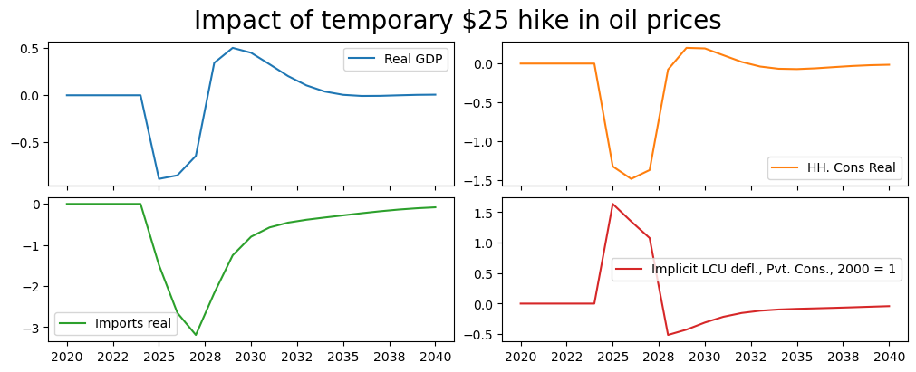
The first variable PAKNYGDPMKTPKN is Pakistan’s real GDP, the second PAKNECONPRVTKN is real consumption, the third is REAL IMPORTS OF GOODS AND SERVICES (PAKNEIMPGNFSKN) and the final is the level of the Consumer price deflator PAKNECONPRVTXN.

The modifier .difpctlevel instructs ModelFlow to calculate the difference in the selected variables and express them as a percent of the original level.

\[ = \frac{x_{new}-x_{original}}{x_{original}} * 100 \]

The modifier rename()will replace the variable name with the variable description in the graphs.

(mpak['PAKNYGDPMKTPKN PAKNECONPRVTKN PAKNEIMPGNFSKN PAKNECONPRVTXN'].
 difpctlevel.rename().plot(title="Impact of temporary $25 hike in oil prices"));

with mpak.set_smpl(2020,2035):
    print(mpak['PAKNYGDPMKTPKN PAKNECONPRVTKN PAKNEIMPGNFSKN PAKNECONPRVTXN'].difpctlevel.df)

      PAKNYGDPMKTPKN  PAKNECONPRVTKN  PAKNEIMPGNFSKN  PAKNECONPRVTXN
2020            0.00            0.00            0.00            0.00
2021            0.00            0.00            0.00            0.00
2022            0.00            0.00            0.00            0.00
2023            0.00            0.00            0.00            0.00
2024            0.00            0.00            0.00            0.00
2025           -0.89           -1.32           -1.49            1.64
2026           -0.85           -1.48           -2.65            1.35
2027           -0.64           -1.37           -3.19            1.08
2028            0.34           -0.08           -2.17           -0.51
2029            0.50            0.20           -1.25           -0.43
2030            0.45            0.19           -0.80           -0.31
2031            0.33            0.11           -0.57           -0.22
2032            0.20            0.02           -0.46           -0.15
2033            0.10           -0.04           -0.39           -0.12
2034            0.04           -0.07           -0.33           -0.10
2035            0.00           -0.07           -0.28           -0.09

The graphs show the change in the level as a percent of the previous level. They suggest that a temporary $25 oil price hike would reduce GDP in the first year by about 0.9 percent, but that the impact would diminish by the third year to -.64 percent, and then turn positive in the fourth year when the temporary price hike was no longer in effect. By the end of the simulation period the net effect on GDP would be zero.

The impacts on household consumption are stronger but follow a similar pattern.

The GDP impact is smaller partly because the decline in domestic demand (due to reduced real incomes from high oil prices) reduces imports. Because imports enter into the GDP identity with a negative sign, a reduction in imports actually increase aggregate GDP – or in this case partially offsets the declines coming from reduced consumption (and investment - which is not shown above).

Finally as could be expected, initially prices rise sharply with higher oil prices. However, as the slowdown in growth is felt, inflationary pressures turn negative and the overall impact on the price level declines. When the oil price hike is eliminated, the overall impact on prices turns negative, and is still slowly returning to zero by the end of the simulation period.

Note: The graph and table above shows what is happening to the price level. To see the impact on inflation (the rate of growth of prices), a separate graph can be generated using difpct, which shows the change in the rate of growth of variables where the growth rate is expressed as a per cent \(\bigg[\bigg(\frac{x^{shock}_t}{x^{shock}_{t-1}}-1\bigg)\) \( - \bigg(\frac{x^{baseline}_t}{x^{baseline}_{t-1}}-1\bigg)\Bigg]*100\).

mpak['PAKNECONPRVTXN'].difpct.rename().plot(
    title="Change in inflation from a temporary $25 hike in oil prices",
                                                   colrow=1,ysize=4);

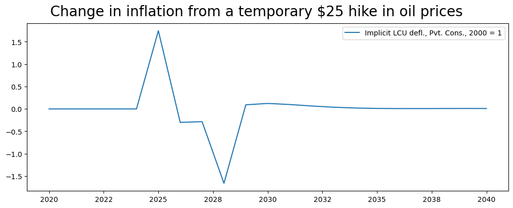
This view, gives a more nuanced result. The inflation rate increases initially by about 1.6 percentage points, but falls compared with the baseline during the 2026-2027 period as the influence of the slowdown in GDP more than offsets the continued inflationary impetus from the lagged increase in oil prices. In 2028, when oil prices drop back to their previous level, an additional dis-inflationary force is generated and a sharp drop in inflation as compared with the baseline ensues. Over time, the boost to demand from lower prices translates into an acceleration in growth and a return of inflation back to its trend rate.

4.2.2. An exogenous shock to a Behavioral variable

Behavioral equations can be de-activated by exogenizing them, either for the entire simulation period, or for a selected sub-period. When exogenized, instead of the equation returning the value returned by its econometrially equation plus the add-factor, it returns the value placed in the variable \(\_X_t\) (see the discussion in Chapter Ten).

In the following scenario, consumption is exogenized for the entire simulation period.

To motivate the simulation, it is assumed that a change in weather patterns has increased the number of sunny days by 10 percent. This increases households happiness and causes them to permanently increase their spending by 2.5% beginning in 2025.

Such a shock can be specified either manually or by using the.fix() method. Below the simpler .fix() method is used, but the equivalent manual steps performed by .fix() are also explained.

To exogenize PAKNECONPRVTKN for the entire simulation period, initially a new DataFrame Cfixed is created as a slightly modified version of mpak.basedf using the .fix() command.

Cfixed=mpak.fix(mpak.basedf,PAKNECONPRVTKN)

This does two things, that could have been done manually. First it sets the dummy variable PAKNECONPRVTKN_D=1 for the entire simulation period. Recall the consumption equation like all behavioral equations of World Bank models implemented in ModelFlowis expressed in two parts.

\[ cons_t= (1-cons\_D)*\bigg[C'(X_t)\bigg] + cons\_D*cons\_X_t\]

When \(cons\_D=1\) (as it does in this scenario) the first part of the equation \((1-cons\_D)*C'(X)\) evaluates to zero and consumption is equal to (1)* \(cons\_X\). If instead (which would be the normal case \(cons\_D\) were set to zero, the equation would simplify to \( cons_t= C'(X_t) \) where \(C'(X_t)\) is the estimated equation that determines the value of real consumption in the model conditioned on the value of other variables in the model (the \(X_t\) of \(C'(X_t)\) and the add factor \(C\_A-t\).

The .fix() method also sets the variable PAKNECONPRVTKN_X in the Cfixed DataFrame equal to the value of PAKNECONPRVTKN in the basedf DataFrame. All the other variables are just copies of their values in .basedf.

With PAKNECONPRVTKN_D=1 throughout the simulation period, the normal behavioral equation is de-activated or exogenized and consumption will just equal its exogenized value: \(PAKNECONPRVTKN=PAKNECONPRVTKN\_X\).

# reset the active sample period to the full model.
mpak.smpl() 
#Create a new df equal to the initial one (bline initialized when we loaded the model) 
# but set real consumption exogenous
Cfixed=mpak.fix(bline,'PAKNECONPRVTKN')

The folowing variables are fixed
PAKNECONPRVTKN

Box 4. The steps performed by the .fix() method

The fix command above effectively does in one line each of the following lines of code.

bline_real=bline.copy() #make a copy of the baseline dataframe

#Create the _X variables if we exogenize the equation
baseline_real = baseline_real.mfcalc('''
PAKNECONPRVTKN_X = PAKNEPRVTKN
''')

#create the _D variable so we can exogenize the equation (set _D=1)-- currently it is exogenized 
baseline_real = baseline_real.upd('''
<-0 -1> 
PAKNECONPRVTKN_D = 1
''')

4.2.2.1. Preparing the shock

For the moment, the equation is exogenized but the values have been set to the same values as the .basedf DataFrame (bline and basedf have the same values on load), so solving the model will not change anything.

The .upd() method can now be used to implement the assumption that real consumption (PAKNECONPRVTKN) would be 2.5% stronger. Because the equation has been turned off, it is the \(\_X\) version of the variable that is increased by 2.5 percent.

# Bump the _X version of the variable by 2.5% between 2025 and 2040
Cfixed=Cfixed.upd("<2025 2040> PAKNECONPRVTKN_X  * 1.025")

4.2.2.2. Performing the simulation

To perform the simulation, the revised CFixed DataFrame is input to the mpak model solve routine, and the model is solved over the period 2020 through 2040.

CFixedRes = mpak(Cfixed,2020,2040,keep='2.5% increase in C 2025-40 (fix)')

# simulates the model for the period 2020 2040 and gives the name '2.5% increase in C 2025-40 to the simulation
CFixedRes = mpak(Cfixed,2020,2040,keep='2.5% increase in C 2025-40') 

The results can be examined graphically as before.

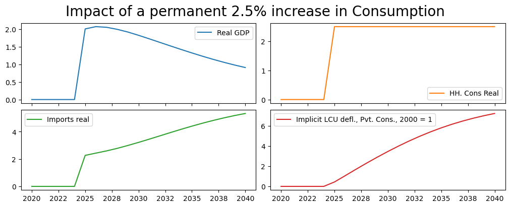
#plots the percent difference (*100) between the lastdf and basedf versions of the specified variables
(mpak['PAKNYGDPMKTPKN PAKNECONPRVTKN PAKNEIMPGNFSKN PAKNECONPRVTXN'].
 difpctlevel.rename().plot(title="Impact of a permanent 2.5% increase in Consumption"));

Below results are displayed in tabular form. Note the use of the pandas options with the with clause. This sets the display format of floating point variables to one decimal points. The second with clause temporarily restricts the display to the period 2020 to 2040.

with pd.option_context('display.float_format', '{:,.1f}%'.format):
    with mpak.set_smpl(2020,2040):
        print(mpak['PAKNYGDPMKTPKN PAKNECONPRVTKN PAKNEIMPGNFSKN'].
              difpctlevel.rename().df)

      Real GDP  HH. Cons Real  Imports real
2020      0.0%           0.0%          0.0%
2021      0.0%           0.0%          0.0%
2022      0.0%           0.0%          0.0%
2023      0.0%           0.0%          0.0%
2024      0.0%           0.0%          0.0%
2025      2.0%           2.5%          2.3%
2026      2.1%           2.5%          2.4%
2027      2.1%           2.5%          2.6%
2028      2.0%           2.5%          2.8%
2029      1.9%           2.5%          3.0%
2030      1.8%           2.5%          3.2%
2031      1.7%           2.5%          3.5%
2032      1.6%           2.5%          3.7%
2033      1.5%           2.5%          3.9%
2034      1.4%           2.5%          4.2%
2035      1.3%           2.5%          4.4%
2036      1.2%           2.5%          4.6%
2037      1.1%           2.5%          4.8%
2038      1.1%           2.5%          5.0%
2039      1.0%           2.5%          5.2%
2040      0.9%           2.5%          5.3%

The permanent rise in consumption by 2.5 percent causes a temporary increase in GDP of about 2% . Higher imports tend to diminish the effect on GDP. Over time higher prices due to the inflationary pressures caused by the additional demand cause the GDP impact to diminish to less than 1 percent by 2040.

4.2.3. Exogenize a behavioral variable and temporarily shock it

The third method of formulating a scenario involves exogenizing an endogenous variable and shocking its value for a defined period of time. The methodology is the same except the period for which the variable is exogenized is different.

Here the set up is basically the same as before.

#reset the active sample period to the full period
mpak.smpl(2020,2040)                                  
# create a copy of the bline DataFrame, but setting the PAKNECONPRVTKN_D variable to 1 for the period 2025 through 2027
CTempExogAll=mpak.fix(bline,'PAKNECONPRVTKN') 

The folowing variables are fixed
PAKNECONPRVTKN

The above .fix() command exogenizes the variable PAKNECONPRVTKN real consumer consumption. The .upd() method in the following line increases the exogenized value of the consumption variable PAKNECONPRVTKN_X by 1.25 percent for three years only, 2025, 2026 and 2027.

# multiply the exogenized value of consumption by 2.5% for 2025 through 2027
CTempExogAll=CTempExogAll.upd("<2025 2027> PAKNECONPRVTKN_X * 1.025")  

Finally the model is solved and selected results displayed as shock-control in percent from the baseline (pre-shock values of the displayed variables).

#Solve the model
CTempXAllRes = mpak(CTempExogAll,2020,2040,keep='2.5% increase in C 2025-27 -- exog whole period') # simulates the model 
(mpak['PAKNYGDPMKTPKN PAKNECONPRVTKN PAKNEIMPGNFSKN PAKNECONPRVTXN'].difpctlevel.
 rename().plot(title="Temporary hike in Consumption 2025-2027"));

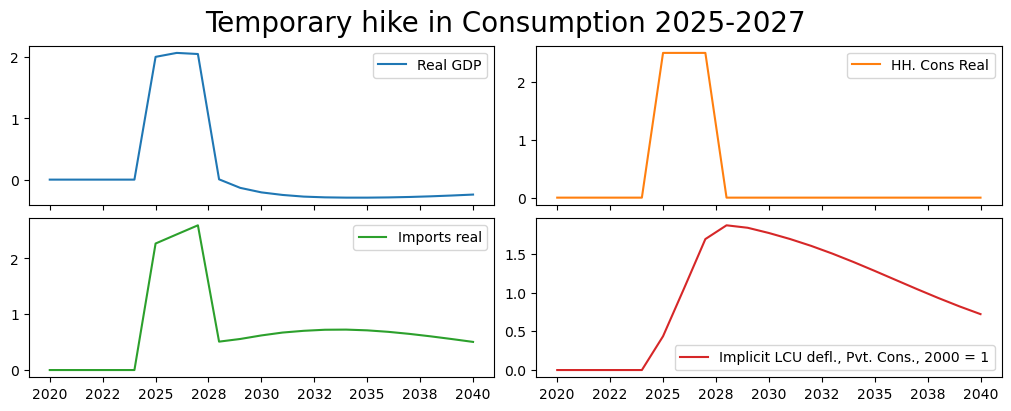
The results are quite different in this scenario. GDP is boosted initially as before but when consumption drops back to its pre-shock level in 2028, GDP and imports decline sharply.

Prices (and inflation) are higher initially but when the economy starts to slow after 2025 prices actually fall (deflation). Although prices are falling, the level of prices remains higher at the end of the simulation than it was in the baseline.

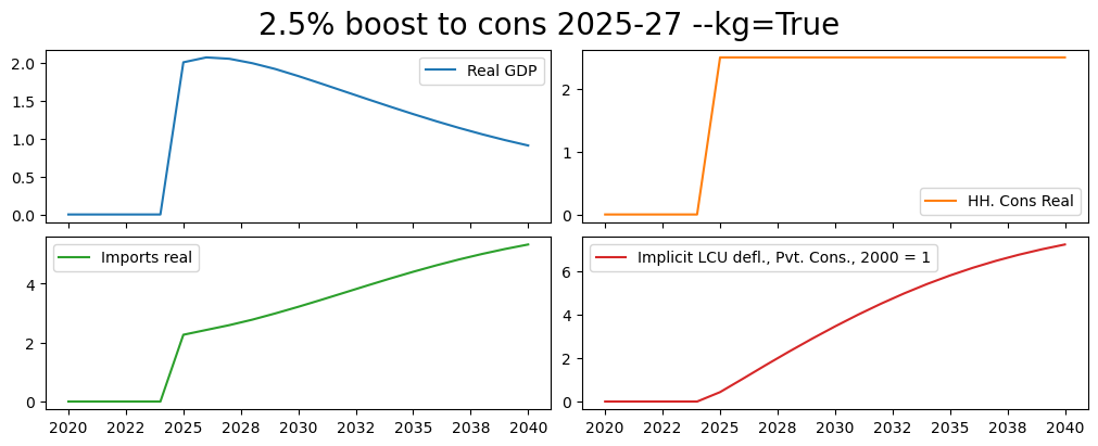
4.2.3.1. Temporary shock exogenized for the whole period (with KG Option)

This scenario is the same as the previous, but this time the --KG (keep_growth) option is used to maintain the pre-shock growth rates of consumption in the post-shock period. Effectively this is the same as a permanent increase in the level of consumption by 2.5% because the final shocked value of consumption (which was 2.5% higher then its pre-shock level) is grown at the same pre-shock rate – ensuring that post-shock the level of consumption remains 2.5% higher in the baseline scenario.

mpak.smpl() # reset the active sample period to the full model.
CTempExogAllKG=mpak.fix(bline,'PAKNECONPRVTKN')
CTempExogAllKG = CTempExogAllKG.upd('''
<2025 2027> PAKNECONPRVTKN_X * 1.025 --kg
''',lprint=0)

#Now we solve the model

CTempXAllResKG = mpak(CTempExogAllKG,2020,2040,keep='2.5% increase in C 2025-27 -- exog whole period --KG=True') # simulates the model 
(mpak['PAKNYGDPMKTPKN PAKNECONPRVTKN PAKNEIMPGNFSKN PAKNECONPRVTXN'].difpctlevel.
 rename().plot(title="2.5% boost to cons 2025-27 --kg=True"));

The folowing variables are fixed
PAKNECONPRVTKN

4.2.4. Exogenize the variable only for the period during which it is shocked

This scenario introduces a subtle but import difference. Here the variable is again exogenized using the fix syntax. But this time it is exogenized only for the period where the variable is shocked.

This means that the consumption equation will only be de-activated for three years (instead of the whole period as in the previous examples). As a result, the values that consumption takes in 2028, 2029, … 2040 depend on the model, not the level it was set to when exogenized (which was the case in the previous scenario).

Looking at the maths of the model the consumption equation is effectively split into three.

1. for the period before 2025 \(cons\_D=0\) and the consumption equation simplifies to:
   \(cons=C(X)\)

2. for the period 2025-2028 it is exogenized (\(cons_D=1\)) so it simplifies to:
   \(cons=cons\_X\)

3. but in the final period 2028-2040 (\(cons\_D=0\)) and the equation reverts to: \(cons=C(X)\)

# reset the active sample period to the full model.
mpak.smpl() 

#Consumption is exogenized only for three years 2025 2026 and 2027 
#     PAKNECONPRVTKN_D=1 for 2025,2026, 2027 0 elsewhere.
# NB the 2025,2027 sets the period over which the change is made not specific dates
# -- i.e. 2025, 2026 and 2027 anot just 2025 and 2027
#In subsequent years (2028 onwards) the level of consumption will be determined by the equation 
CExogTemp=mpak.fix(bline,'PAKNECONPRVTKN',2025,2027)

#Now increase Consumption by 2.5% over the period 2025-2027
CExogTemp = CExogTemp.upd('<2025 2027> PAKNECONPRVTKN_X * 1.025',lprint=0)       

#Solve the model by passing it the revised DataFrame
CExogTempRes = mpak(CExogTemp,2020,2040,keep='2.5% increase in C 2025-27 -- temporarily exogenized') # simulates the model 


#display the impulse response functions of the specified variables
(mpak['PAKNYGDPMKTPKN PAKNECONPRVTKN PAKNEIMPGNFSKN PAKNECONPRVTXN'].difpctlevel.
rename().plot(title="Temporary 2.5% boost to cons 2025-27 - equation active"));

The folowing variables are fixed
PAKNECONPRVTKN

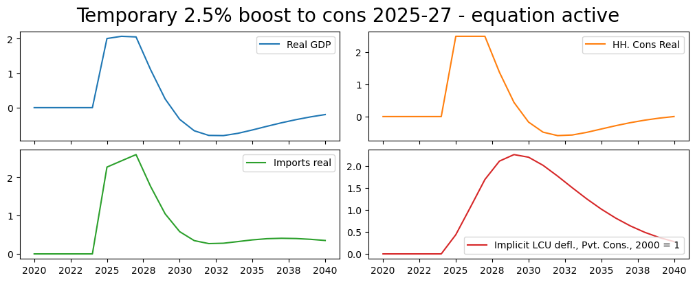
These results have important differences compared with the previous. The most obvious is visible in looking at the graph for Consumption. Rather than reverting immediately to its earlier pre-shock level, it falls more gradually and actually overshoots (falls below its earlier level), before returning slowly to its pre-shock level. That is because unlike in the previous shocks, its path after 2027 is being determined endogenously and reacting to changes elsewhere in the model, notably changes to prices, wages and government spending as well as the lagged level of consumption.

print('Consumption base and shock levels\r\n');

print('\r\nReal values in 2030');
print(f'Base value:  {bline.loc[2028,"PAKNECONPRVTKN"]:,.0f}.\tShocked value: {CExogTempRes.loc[2028,"PAKNECONPRVTKN"]:,.0f}.\r\n'
    f'Percent difference: {round(100*((CExogTempRes.loc[2030,"PAKNECONPRVTKN"]-bline.loc[2028,"PAKNECONPRVTKN"])/bline.loc[2028,"PAKNECONPRVTKN"]),2)}')
print('\r\n\r\nReal values in 2040');
print(f'Base value:  {bline.loc[2040,"PAKNECONPRVTKN"]:,.0f}.\tShocked value: {CExogTempRes.loc[2040,"PAKNECONPRVTKN"]:,.0f}.\r\n'
    f'Percent difference: {round(100*((CExogTempRes.loc[2040,"PAKNECONPRVTKN"]-bline.loc[2040,"PAKNECONPRVTKN"])/bline.loc[2040,"PAKNECONPRVTKN"]),2)}')

Consumption base and shock levels


Real values in 2030
Base value:  27,241,278.	Shocked value: 27,616,949.
Percent difference: 5.36


Real values in 2040
Base value:  38,692,815.	Shocked value: 38,693,167.
Percent difference: 0.0

4.2.5. Simulation with Add factors

Add factors are a crucial element of the macromodels of the World Bank and serve multiple purposes.

In simulation, add-factors allow simulations to be conducted without de-activating behavioral equations. Such shocks are often referred to as endogenous shocks because the equation of the behavioral variable that is shocked remains active throughout.

In some ways they are very similar to a temporary exogenous shock. Both ways of producing the shock allow the shocked variable to respond endogenously in the period after the shock. The main difference between the two approaches is in an endogenous shock (add-factor shock), the equation remains active throughout, including during the period the variable is being shocked.

The intuition here for our previous consumption example might be that animal spirits cause households to increase consumption by 2.5 percent all things equal. However, all things are not equal – GDP is higher employment demand is higher which would boost consumption even more; but inflation is also higher which would reduce real incomes and supress consumption. The net effect will balance these three (and other) factors out even in the shock period.

Box 5. Endogenous (Add-factor) shocks versus temporarily exogenized shocks

• Endogenous shocks (Add-Factor shocks) allow the shocked variable to respond to changed circumstances that occur during the period of the shock.

  • This approach makes most sense for “animal spirits”, shocks where the underlying behavior is expected to change.

  • It also makes sense when actions of one part of an aggregate is likely to impact behavior of other sectors within an aggregate.

    • Increased investment by a particular sector would be an example here as the associated increase in activity is likely to increase investment incentives in other sectors, while increased demand for savings will increase interest rates and the cost of capital operating in the opposite direction.

    • The final simulation level of the shocked variable during the period of the shock will be equal to the original level plus the shock, plus whatever endogenous additional changes in the shocked variable arise because the conditioning variables (the \(X_t\) in the equation) change.

• Exogenous shocks to endogenous variables fix the level of the shocked variable during the shock period.

  • Changes in government spending policy, something that is often largely an economically exogenous decision.

  • the final simulation level of the shocked variable during the period of the shock will be exactly equal to the original level plus the shock

4.2.5.1. Simulating the impact of a planned investment

The following simulation uses the add-factor to simulate the impact of a 3 year investment program beginning in 2025 of 1 percent of GDP per year. This might reflect a specific large scale plant that is being constructed due to a deal reached by the government with a foreign manufacturer. The add-factor approach is chosen because the additional investment is likely to increase demand for the products of other firms, which is likely to incite them to add to their investments as well – both after the shock as in previous examples but also during the period that investment is being shocked.

4.2.5.1.1. How to translate the economic shock into a model shock

Add-factors in the MFMod framework are applied to the intercept of an equation (not the level of the dependent variable). This preserves the estimated elasticities of the equation, but makes introduction of an add-factor shock somewhat more complicated than the exogenous approach. Below a step-by-step how-to guide:

1. Identify numerical size of the shock

2. Examine the functional form of the equation, to determine the nature of the add factor. If the equation is expressed as a:

   • growth rate then the add-factor will be an addition or subtraction to the growth rate

   • percent of GDP (or some other level) then the add-factor will be an addition or subtraction equal to the desired shock expressed as a percent of pre-shock GDP.

   • Level then the add-factor will be a direct addition to the level of the dependent variable

3. Convert the economic shock into the units of the add-factor

4. Shock the add-factor by the above amount and run the model

Note

The add-factor is an exogenous variable in the model, so shocking it follows the well-established process for shocking an exogenous variable.

4.2.5.1.2. Determine the size of shock

Above the shock was identified as a 1 percent of GDP increase in private-sector investment. A first step would be to determine the variable(s) that need to be shocked — private investment. To do this we can query the variable dictionary, in this case by listing all variables where invest is part of the variable description.

Note

Variable selection
More on how to use wildcards to select variables can be found at Variable selection with wildcharts

mpak['!*invest*'].des

PAKNEGDIFGOVKN        : Pub investment real
PAKNEGDIFPRVKN        : Prvt. Investment real
PAKNEGDIFPRVKN_A      : Add factor:Prvt. Investment real
PAKNEGDIFPRVKN_D      : Fix dummy:Prvt. Investment real
PAKNEGDIFPRVKN_FITTED : Fitted  value:Prvt. Investment real
PAKNEGDIFPRVKN_X      : Fix value:Prvt. Investment real
PAKNEGDIFTOTKN        : Investment real

Querying for all variables that “invest” in their descriptor gives us the mnemonic for the private investment variable PAKNEGDIFPRVKN.

4.2.5.1.3. Identify the functional form(s)

To understand how to shock using the add factor, it is essential to understand how the add-factor enters into the equation.

Addfactor is on the intercept of	Shock needs to be calculated as
a growth equation	a change in the growth rate
Share of GDP	a percent of GDP
Level	as change in the level

Use the .eviews command command to identify the functional forms of the equation to be shocked.

mpak['PAKNEGDIFPRVKN'].eviews

PAKNEGDIFPRVKN : 
(PAKNEGDIFPRVKN/PAKNEGDIKSTKKN( - 1)) = 0.00212272413966296 + 0.970234989019907*(PAKNEGDIFPRVKN( - 1)/PAKNEGDIKSTKKN( - 2)) + (1 - 0.970234989019907)*(DLOG(PAKNYGDPPOTLKN) + PAKDEPR) + 0.0525240494260597*DLOG(PAKNEKRTTOTLCN/PAKNYGDPFCSTXN)

In this case the equation is written as a share of the capital stock in the preceding period PAKNEGDIKSTKKN(-1).

4.2.5.1.4. Calculate the size of the required add factor shock

The shock to be executed is 1.0 percent of GDP.

It is assumed that the money will be spent in one year on private investment.

The private investment equation is written as a share of the capital stock lagged one period. Therefore, the add-factor needs to be shocked by adding 1 percent of GDP to private investment in 2028 divided by the capital stock in 2027.

#Create a DataFrame AFShock that is equal tothe baseline
AFShock=bline

#Display the level of the AF
print("Pre shock levels")
AFShock.loc[2025:2030,['PAKNEGDIFPRVKN_A','PAKNEGDIFPRVKN','PAKNEGDIKSTKKN']]

#print(AFShock.loc[2025:2030,'PAKNEGDIFPRVKN']/AFShock.loc[2025:2030,'PAKNYGDPMKTPKN']*100)

Pre shock levels

	PAKNEGDIFPRVKN_A	PAKNEGDIFPRVKN	PAKNEGDIKSTKKN
2025	-0.00	1602853.65	47303916.21
2026	-0.00	1581104.20	48148785.83
2027	-0.00	1569541.20	49009798.90
2028	-0.00	1569140.97	49898686.55
2029	-0.00	1580576.85	50826938.84
2030	-0.00	1604394.55	51805897.58

Below the mfcalc routine is used to set the addfactor variable equal to its previous value plus the equivalent of 1 percent of GDP when expressed as a percent of the previous period’s level of capital stock.

AFShock=AFShock.mfcalc("""
 <2028 2028> PAKNEGDIFPRVKN_A = PAKNEGDIFPRVKN_A +(.01*PAKNYGDPMKTPKN/PAKNEGDIKSTKKN(-1))
 """);

print("Shocked AF levels")
AFShock.loc[2025:2030,'PAKNEGDIFPRVKN_A']

Shocked AF levels

2025   -0.00
2026   -0.00
2027   -0.00
2028    0.01
2029   -0.00
2030   -0.00
Name: PAKNEGDIFPRVKN_A, dtype: float64

4.2.5.1.5. Run the shock

The shock is executed by submitting the revised dataframe to the model object, and solving the model over the period 2020 through 2040.

# the simulation is done until 2050, for later use of the keept values
AFShockRes = mpak(AFShock,2020,2050,keep='1% of GDP increase in FDI and private investment (AF shock)')
mpak.smpl(2020,2035)
(mpak['PAKNYGDPMKTPKN PAKNEGDIFPRVKN PAKNECONPRVTKN PAKNEIMPGNFSKN PAKNEGDIFTOTKN PAKNECONPRVTXN'].
 difpctlevel.rename().plot(title="Add factor shock on private investment 1% of GDP"));

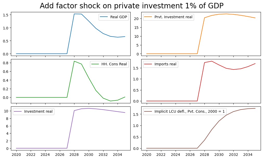
The above graphs are expressed as a percent of the baseline value of each value. Because private investment in the baseline is only 5 percent of GDP, the 1% of GDP shock, expressed as a percent of private investment is much larger (about 20 times larger).

Below to double-check the calculations, two variables IFPRVOLD_ORIG and IFTOT_ORIG are created that reflect pre-shock private and total investment as a share of pre-shock GDP. Two additional variables IFPRV_SHOCK and IFTOT_SHOCK are also created as the shocked values of private and total investment as a percent of the original GDP. The difference between the two sets of variables is the increase in fixed private and fixed total investment as a percent of the same denominator (the original level of GDP).

The ex-post change in private investment and of total investment in 2028 is 1.06 and 1.11 percent respectively, 0.6 and 1.1 percentage points larger than the actual shock 1 percent of GDP shock to the addfactor.

This difference represents the endogenous reaction of other investors in the same time period to the changed circumstances. It is precisely to capture this effect that an endogenous or add-factor shock is employed.

AFShockRes['GDPOLD']=bline['PAKNYGDPMKTPKN']
AFShockRes['IFPRVOLD']=bline['PAKNEGDIFPRVKN']
AFShockRes['IFTOTOLD']=bline['PAKNEGDIFTOTKN']
AFShockRes=AFShockRes.mfcalc('''
                       IFPRV_SHOCK = PAKNEGDIFPRVKN / GDPOLD*100
                       IFTOT_SHOCK = PAKNEGDIFTOTKN / GDPOLD*100
                       IFPRV_Orig = IFPRVOLD / GDPOLD*100
                       IFTOT_Orig = IFTOTOLD / GDPOLD*100
                       IFPRV_IMPACT = IFPRV_SHOCK - IFPRV_Orig
                       IFTOT_IMPACT = IFTOT_SHOCK - IFTOT_Orig

                       ''')

print(round(AFShockRes.loc[2025:2030,['IFPRV_ORIG','IFPRV_SHOCK',
                                      'IFTOT_ORIG','IFTOT_SHOCK', 
                                      'IFPRV_IMPACT', 'IFTOT_IMPACT']],2))

      IFPRV_ORIG  IFPRV_SHOCK  IFTOT_ORIG  IFTOT_SHOCK  IFPRV_IMPACT  IFTOT_IMPACT
2025        5.73         5.73       11.31        11.31          0.00          0.00
2026        5.52         5.52       11.21        11.21          0.00          0.00
2027        5.34         5.34       11.12        11.12          0.00          0.00
2028        5.19         6.25       11.05        12.16          1.06          1.11
2029        5.08         6.19       11.01        12.17          1.10          1.16
2030        5.01         6.13       10.99        12.16          1.12          1.17

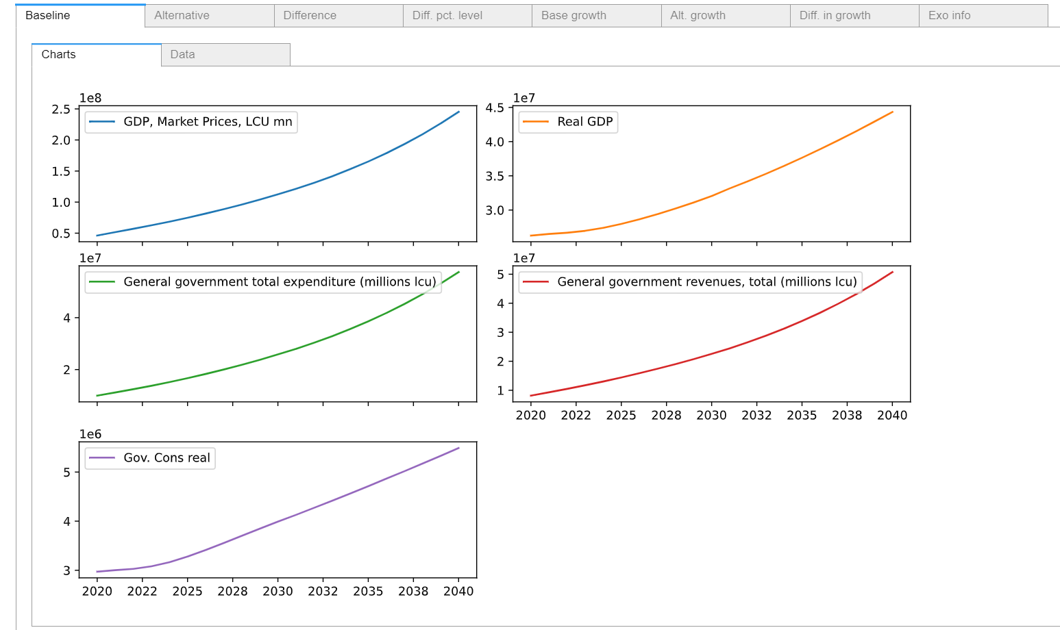
4.3. The results visualization widget view

When working in Jupyter Notebook, referencing a selection of series will cause a data visualization widget to be generated that allows you to look at results (basesdf vs latestdf) for the selected variables as tables or charts, as levels, as growth rates and as percent differences from baseline.

display(mpak['PAKNYGDPMKTPCN PAKNYGDPMKTPKN PAKGGEXPTOTLCN PAKGGREVTOTLCN PAKNECONGOVTKN'])

4.4. Save simulation results to a pcim file for later exploration

The next chapter explores the different results generated during these simulations. Rather than re-run them, the model object mpak (and the simulation results that are stored by the keep command used above) are saved to a local file for retrieval in the next chapter.

NB: The keep=True instructs ModelFlow to save the results from any kept solutions as well.

help(mpak.modeldump)

Help on method modeldump in module modelclass:

modeldump(file_path='', keep=False, zip_file=True) method of modelclass.model instance

mpak.modeldump(r'../models/mpakw.pcim',keep=True)

mpak.keep_solutions.keys() 

dict_keys(['Baseline', '$25 increase in oil prices 2025-27', '2.5% increase in C 2025-40', '2.5% increase in C 2025-27 -- exog whole period', '2.5% increase in C 2025-27 -- exog whole period --KG=True', '2.5% increase in C 2025-27 -- temporarily exogenized', '1% of GDP increase in FDI and private investment (AF shock)'])

---

[1]

If a model does not reproduce itself when solved, then mathematically it means that the system of equations is not closed (there is no single answer) or data are inconsistent (usually one or more identities do not hold). In such circumstances, either the model will not solve or it will but it will not be possible to have confidence in any of the results generated.