Working with a World Bank Model under ModelFlow

2. Working with a World Bank Model under ModelFlow#

The basic method for working with any model is the same. Indeed the initial steps followed here are the same as were followed during the preceding discussions of ModelFlow features.

Process:

Prepare the workspace
Load the model ModelFlow
Design some scenarios
Simulate the model
Visualize the results

2.1. Prepare the work space#

To use ModelFlow it must be installed as per the instructions in Chapter 3 (a one-time operation). The the python environment into which ModelFlow was installed must be activated. For users that installed ModelFlow according to the earlier instructions this can be achieved by executing conda activate ModelFlow in line with earlier instructions.

Once the python environment is activated, the ModelFlow and pandas packages must be imported into your workspace. Once this is done (accomplished by the code below), the user is ready to work with ModelFlow.

In this chapter - Working with a World Bank Model under ModelFlow

This chapter provides practical guidance on using World Bank models within the ModelFlow framework.

Key points include:

Setup and Preparation:
- Prepare the workspace by setting up the Python environment.
- Load the model, associated data, and variable descriptions.
Model Exploration:
- Extract information about the model, including:
  - its equations
  - its variables
  - its structure
  - its data
- Organize variables into groups for streamlined exploration and analysis.
Key Methods:
- Use ModelFlow’s built-in functions to query, modify, and analyze data.
- Explore relationships between variables and their role in the model.

# Prepare the notebook for use of ModelFlow 

# Jupyter magic command to improve the display of charts in the Notebook
%matplotlib inline

# Import pandas 
import pandas as pd

# Import the model class from the modelclass module 
from modelclass import model 

# functions that improve rendering of ModelFlow outputs
model.widescreen()
model.scroll_off();

2.2. Load the model: Load a pre-existing model, data and descriptions#

To load a model use the model.modelload() method of ModelFlow. In the example below, the model has been saved to the models folder located one level above the directory from which the Jupyter Notebook has been executed (but within the scope of Jupyter itself, i.e. below the directory from which the Jupyter system was launched.

2.2.1. The `.modelload()` method#

The command below

mpak,bline = model.modelload('../models/pak.pcim', alfa=0.7,run=1,keep= 'Baseline')

instantiates (creates an instance of) a ModelFlow model object using the model object (equiations and data) contained in the file pak.pcim and assigns it to the variable name mpak.

The run=1 option executes the model and assigns the result of the model execution to the DataFrame bline.

The model is solved with the parameter alfa set to 0.7. The \(alfa \in (0,1)\) parameter determines the step size of the solution engine. The larger alfa the larger the step size. Larger step sizes solve faster, but may have trouble finding a unique solution. Smaller step sizes take longer to solve but are more likely to find a unique solution. Values of alfa=.7 work well for World Bank models.

The keep option instructs ModelFlow to maintain in the model object (mpak) the results of the initial scenario, assigning it the text name Baseline. As written, modelload returns both the model object mpak, but also a DataFrame bline that is assigned the results of the simulation. This DataFrame is distinct from the one that is stored inside the mpak model object by the keep= command, although the data inside each of these DataFrames will have the same numerical values. The keep option is described in more detail in the following chapter on scenarios.

Warning

If ModelFlow cannot find the file at the position indicated it will look for it in the global Model repository on line.

Upon return, the modelload command indicates the location from which the model was retrieved. In this case, from the requested local file store.

#Replace the path below with the location of the pak.pcim file (or some other world bank model file) on your computer
mpak,bline = model.modelload('../models/pak.pcim', \
                                alfa=0.7,run=1,keep= 'Baseline')

Zipped file read:  ..\models\pak.pcim

2.2.2. Extracting information about the model#

The newly loaded python object mpak is an instance of the model class and as such inherits the methods (functions) and properties (data) of that class. To learn about the model there are a variety of methods that can be used to extract information about the model and its data.

A World Bank model in ModelFlow contains a wide range of objects.

variables – time series variables comprised of mnemonics and data
dataframes – data for each variable generated in different simulations
groups – lists of variables
equations – identities and behaviorals
model – the model object itself

Extracting information about each of these objects is central to working with WBG models in ModelFlow.

The model object contains information about the model itself, its name, its structure (does it contain simultaneous equations or is it recursive), the number of variables it contains and the number that are exogenous and endogenous (have associated equations). Executing the unadorned name of a model object, i.e. mpak displays summary information about the model object.

mpak

<
Model name                              :                  PAK 
Model structure                         :         Simultaneous 
Number of variables                     :                  839 
Number of exogeneous  variables         :                  461 
Number of endogeneous variables         :                  378 
>

The model work space also has a time dimension, its sample period. This can be retrieved and changed.

mpak.current_per

Index([2016, 2017, 2018, 2019, 2020, 2021, 2022, 2023, 2024, 2025, 2026, 2027,
       2028, 2029, 2030, 2031, 2032, 2033, 2034, 2035],
      dtype='int64')

Here the model is currently set up to solve over the period 2016 through 2030. That period can be changed assuming, as is the case with the Pakistan model, that additional data are available.

2.2.3. Information about variables#

The model object mpak contains lists of all the variables that form part of the model, and these lists can be interrogated to garner information about the model. The Table below indicates some of the most important of these queries. The variables for which information is sought can be specified directly or through a wildcard specification (see note).

Method	Example	Information returned
`.names`	`mpak ['PAKNECON*XN] .name`	A python list of the mnemonics of all the variables defined and contained in the model object that match the search paremers in the `[]`
`.des`	`mpak ['PAKNECONPRVT?N'] .des`	A dictionary of mnemonics and their variable descriptions
`.<var name>.show`	`mpak.PAKNECONPRVTXN.show`	Lists the equation (formula), variable descriptions and data values of a specific variable

Note

Wildcards

Most of the variable and equation information commands accept wildcard specifications in the search parameter.

The * character in the command mpak['PAKNECON*XN'].names example is a wildcard character and the expression will return all variables that begin PAKNECON and end XN.

The ? in the .des example is another wildcard expression. It will match only single characters. Thus mpak['PAKNECONPRVT?N'].names would return three variables: PAKNECONPRVTKN, PAKNECONPRVTXN, and PAKNECONPRVTXN. The real, current value, and deflators for household consumption expenditure.

Note the final show example uses a slightly different syntax where the variable to be operated upon is specified directly: modelname.PAKNECONPRVTXN.show.

The example below returns the mnemonics and descriptions of all variables matching the pattern PAKNYGDP*KN, i.e. Pakistani variables (PAK) from the National Income Accounts (NY) from the main sub-category GDP that are also real (K) expressed in local currency units (N) variables.

Box 3. World Bank Mnemonics

A typical World Bank model will have in excess of 300 variables. Each has a mnemonic typically comprised of 14 characters that is structured in a specific way, The root for almost all variables is the three letters of the ISO code for the country to which the variable pertains. Other letters describe the variable in ever finer detail (see below).

\[\texttt{12345678901234}\]

\[\color{green}{\texttt{CCC}}\color{red}{\texttt{AA}}\color{lime}{\texttt{MMM}}\color{blue}{\texttt{NNNN}}\color{magenta}{\texttt{U}}\color{black}{\texttt{C}}\]

where:

Letters	Meaning
\(\color{green}{\texttt{CCC}}\)	The three-leter ISO code for a country – i.e. IDN for Indonesia, RUS for Russia
\(\color{red}{\texttt{AA}}\)	The two-letter major accounting system to which the variable attaches (see following Table for more info)
\(\color{lime}{\texttt{MMM}}\)	The three-letter major sub-category of the data - i.e. GDP, EXP - expenditure
\(\color{blue}{\texttt{NNNN}}\)	The four-letter minor sub-category MKTP for market prices
\(\color{magenta}{\texttt{U}}\)	The measure (K: real variable;C: Current Values; X: Prices)
\(\color{black}{\texttt{C}}\)	denotes the Currency (N: National currency; D: USD; P: PPP)

Common major accounting systems mnemonics:

The, \(\color{red}{\texttt{AA}}\)s from above include:

Code	Meaning
NY	National income
NE	National expenditure Accounts
NV	Value added accounts
GG	General Government Accounts
BX	Balance of Payments: Exports
BM	Balance of Payments: Imports
BN	Balance of Payments: Net
BF	Balance of Payments: Financial Account

Less common terminations: Occasionally you will see variables with and ‘_’ appended to the name. This indicates that the variable is being expressed as a percent of something (usually GDP). Thus PAKBNCABFUNDCD_ means Pakistan (PAK) Balance of Payments, net (BN) of the Current Account (CAB) IMF definition (FUND) in Current (C) Dollars (D) expressed as a percent of GDP.

Others less common terminations include ER (Effective rate) and (SR) Statutory rate used to denote the average tax rate (ER) of a tax versus the legal rate (SR).

Thus:

Mnemonic	Meaning
IDNNYGDPMKTPKN	Indonesia GDP at market prices, real in Indonesian Rupiah
KENNECPNPRVTXN	Kenya Private (household) consumption expenditure schillings deflator
BOLGGEXPGNFSCN	Bolivia Government Expenditure on Goods and services (GNFS) in current Bolivars
HRVGGREVDCITCN	Croatia Government Revenues Direct Corporate Income Taxes in current Euros
NPLBXGSRNFSVCD	Nepal BOP Exports of non-factor services (goods and services) in current USD

If executed, the command mpak['*'].des would return a dictionary of all the mnemonics and descriptions of all the variables in the mpak model object.

The below command is more restrictive and returns only the variables that start PAKNYGDP and KN.

mpak['PAKNYGDP*KN'].des

PAKNYGDPDISCKN : GDP Disc., 2000 LCU mn
PAKNYGDPFCSTKN : GDP Factor Cost Local Currency units Volumes National base year
PAKNYGDPMKTPKN : Real GDP
PAKNYGDPPOTLKN : Potential Output, constant LCU

2.2.3.1. The `!` operator – searching on the variable description#

The ! operator allows the same methods to be used to retrieve information about variables, but based on their descriptions. Pre-pending the search string with the ! operator, tells it to try and match (and display) information about variables based on their descriptions not their mnemonics.

Note

The ! operator

If a wildcard is preceded by an exclamation mark ! the search will be done over the description of variables instead of the mnemonic

The below expression returns the mnemonics of all variables whose description includes the word Carbon.

mpak['!*Carbon*'].names

['PAKCCEMISCO2TKN', 'PAKGGREVCO2CER', 'PAKGGREVCO2GER', 'PAKGGREVCO2OER']

The following expression returns the mnemonics and descriptions of the same variables.

mpak['!*Carbon*'].des

PAKCCEMISCO2TKN : Total Carbon emissions (tons)
PAKGGREVCO2CER  : Carbon tax on coal (USD/t)
PAKGGREVCO2GER  : Carbon tax on gas (USD/t)
PAKGGREVCO2OER  : Carbon tax on oil (USD/t)

The following expression returns the descriptions of a specific variable.

mpak.var_description['PAKGGREVCO2OER']

'Carbon tax on oil (USD/t)'

2.3. Groups#

ModelFlow incorporates a variant of the idea of groups from EViews. In ModelFlow the groups defined in an imported EViews workfile are converted into entries in a dictionary called var_groups which can be interrogated, added to and amended like any dictionary in python.

The command mpak.var_groups will return all of the groups already defined in mpak.

mpak.var_groups

{'Headline': '{cty}NYGDPMKTPKN {cty}NYGDPMKTPXN {cty}NRTOTLCN {cty}LMUNRTOTLCN {cty}BFFINCABDCD  {cty}BFBOPTOTLCD {cty}GGBALEXGRCN {cty}GGDBTTOTLCN_ {cty}GGDBTTOTLCN {cty}BNCABLOCLCD_ {cty}FPCPITOTLXN {cty}CCEMISCO2TKN',
 'National income accounts': '{cty}NY*',
 'National expenditure accounts': '{cty}NE*',
 'Value added accounts': '{cty}NV*',
 'Balance of payments exports': '{cty}BX*',
 'Balance of payments exports and value added ': '{cty}BX* {cty}NV*',
 'Balance of Payments Financial Account': '{cty}BF*',
 'General government fiscal accounts': '{cty}GG*',
 'World all': 'WLD*',
 'All variables': '*'}

A group can be added to the dictionary by giving it a unique identifier (key) and associating with it a string defining the group, using a wildcard specification or just a space de-limited list of mnemonics.

Thus the first command below will generate a new group called ‘MyGroup’ that contains all variables beginning PAKGGREV and ending CN, plus the variable PAKGGBALOVRLCN to the dictionary var_groups that is part of the model object mpak. The second creates a group called LaborMarket which contains the variables for Employment and the Unemployment rate.

mpak.var_groups['MyGroup']='PAKGGREV*CN PAKGGBALOVRLCN'
mpak.var_groups['LaborMarket']='PAKLMEMPTOTLCN PAKLMUNRTOTLCN'

2.3.1. The `#` operator – searching on the variable description#

The # operator allows the same methods to be used to retrieve information about groups. Pre-pending the search string with the # operator, tells it to try and match (and display) information about the variables in groups that match the search expression following the #.

Note

The # operator

If a wildcard is preceded by an exclamation mark # the search will be done over the groups in the model object and will return information about the members of the returned groups

The below expression returns the mnemonics of all variables that are a member of the MyGroup Group.

mpak['#MyGroup'].names

['PAKGGREVDRCTCN',
 'PAKGGREVEMISCN',
 'PAKGGREVGNFSCN',
 'PAKGGREVGRNTCN',
 'PAKGGREVOTHRCN',
 'PAKGGREVTOTLCN',
 'PAKGGREVTRDECN',
 'PAKGGBALOVRLCN']

2.3.2. Information about the data of series in a group#

The unadorned command mpak[#MyGroups] invokes a widget that shows all of the data in the group MyGroup and various representations (level and growth rates) both as tables and charts.

mpak['#MyGroup']

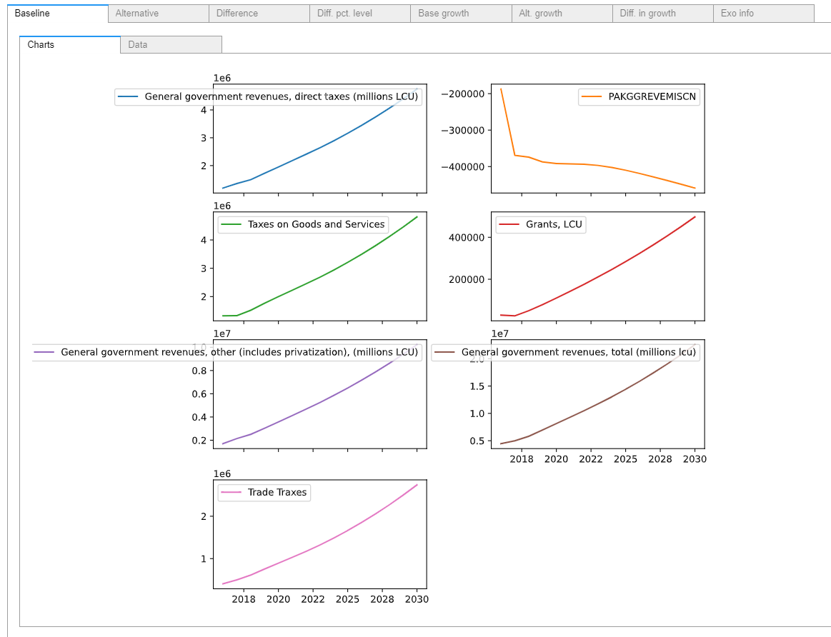
Alternatively just the graphs and or tables can be returned, by appending the .df method (tables) or .plot() methods (charts). Modifying the command further by including the .pct command would display the data as growth rates.

mpak['#MyGroup'].df

	PAKGGREVDRCTCN	PAKGGREVEMISCN	PAKGGREVGNFSCN	PAKGGREVGRNTCN	PAKGGREVOTHRCN	PAKGGREVTOTLCN	PAKGGREVTRDECN	PAKGGBALOVRLCN
2016	1.192249e+06	-187487.145911	1.319524e+06	28696.665825	1.704982e+06	4.463113e+06	4.051485e+05	-1.322586e+06
2017	1.354036e+06	-368998.340503	1.327860e+06	25349.188671	2.141104e+06	4.976845e+06	4.974946e+05	-1.833428e+06
2018	1.492389e+06	-373989.822891	1.516485e+06	49838.249131	2.505467e+06	5.802066e+06	6.118760e+05	-1.814775e+06
2019	1.721883e+06	-387328.506687	1.764865e+06	78978.628390	3.033525e+06	6.967846e+06	7.559233e+05	-1.764188e+06
2020	1.950849e+06	-391591.258722	1.998747e+06	110163.222890	3.574406e+06	8.136424e+06	8.938484e+05	-1.798450e+06
2021	2.178938e+06	-392424.135886	2.225111e+06	142678.758699	4.122857e+06	9.307621e+06	1.030460e+06	-1.857821e+06
2022	2.407303e+06	-393527.268710	2.450129e+06	176071.658354	4.677542e+06	1.048922e+07	1.171700e+06	-1.939507e+06
2023	2.644233e+06	-396768.489162	2.685256e+06	210616.945645	5.252367e+06	1.171840e+07	1.322695e+06	-2.033015e+06
2024	2.894933e+06	-402416.006307	2.936720e+06	246606.677324	5.856855e+06	1.301870e+07	1.486000e+06	-2.146245e+06
2025	3.161598e+06	-409971.057281	3.206328e+06	284195.083320	6.495230e+06	1.439974e+07	1.662364e+06	-2.279101e+06
2026	3.444363e+06	-418754.040372	3.493313e+06	323384.807252	7.167704e+06	1.586160e+07	1.851585e+06	-2.433659e+06
2027	3.743124e+06	-428241.872484	3.796738e+06	364156.630890	7.874000e+06	1.740321e+07	2.053431e+06	-2.610006e+06
2028	4.058704e+06	-438151.424003	4.116861e+06	406583.540873	8.615802e+06	1.902797e+07	2.268174e+06	-2.806904e+06
2029	4.393195e+06	-448385.655807	4.455458e+06	450879.142260	9.397577e+06	2.074544e+07	2.496720e+06	-3.022765e+06
2030	4.749689e+06	-458938.010233	4.815425e+06	497380.152375	1.022607e+07	2.257011e+07	2.740488e+06	-3.256688e+06
2031	5.131800e+06	-469817.783803	5.200188e+06	546498.760163	1.110928e+07	2.451915e+07	3.001198e+06	-3.508801e+06
2032	5.543290e+06	-481016.427390	5.613280e+06	598678.767743	1.205564e+07	2.661059e+07	3.280716e+06	-3.780096e+06
2033	5.987899e+06	-492506.888551	6.058177e+06	654372.159746	1.307361e+07	2.886255e+07	3.580994e+06	-4.072057e+06
2034	6.469364e+06	-504258.235259	6.538358e+06	714036.436715	1.417167e+07	3.129327e+07	3.904098e+06	-4.386355e+06
2035	6.991538e+06	-516250.612903	7.057461e+06	778144.673255	1.535858e+07	3.392175e+07	4.252273e+06	-4.724724e+06

Below the same logic is used to display the data from variables matching a mnemonic search. The results have been placed inside a with mpak.set_smpl() clause to restrict the output to a shorter period. If it was not used the output would cover the whole time period of the .lastdf DataFrame from which all of these data are drawn.

Note

When using a with clause, an explicit print statement is required.

with mpak.set_smpl(2020,2025):
    print(round(mpak['#MyGroup'].pct.df,2)) # round restricts the display to 2 decimal points

      PAKGGREVDRCTCN  PAKGGREVEMISCN  PAKGGREVGNFSCN  PAKGGREVGRNTCN  \
         13.30            1.10           13.25           39.48   
         11.69            0.21           11.33           29.52   
         10.48            0.28           10.11           23.40   
          9.84            0.82            9.60           19.62   
          9.48            1.42            9.36           17.09   
          9.21            1.88            9.18           15.24   

      PAKGGREVOTHRCN  PAKGGREVTOTLCN  PAKGGREVTRDECN  PAKGGBALOVRLCN  
         17.83           16.77           18.25            1.94  
         15.34           14.39           15.28            3.30  
         13.45           12.69           13.71            4.40  
         12.29           11.72           12.89            4.82  
         11.51           11.10           12.35            5.57  
         10.90           10.61           11.87            6.19  

When displaying a dataframe or a manipulation of a dataframe in cases where the output might include very many lines of output, Jupyter will, by default, truncate the output by showing the first and last five observations of the active sample period when the same call is made without the with clause.

mpak.smpl(2000,2100)  # change the default view to cover 100 observations
round(mpak['#MyGroup'].pct.df,2)  #Jupyter will truncate the output

	PAKGGREVDRCTCN	PAKGGREVEMISCN	PAKGGREVGNFSCN	PAKGGREVGRNTCN	PAKGGREVOTHRCN	PAKGGREVTOTLCN	PAKGGREVTRDECN	PAKGGBALOVRLCN
2000	9.55	101.83	70.02	NaN	NaN	7.30	-21.68	15.14
2001	11.14	15.37	31.46	inf	inf	16.34	5.52	-35.57
2002	14.66	-13.23	8.55	94.82	17.59	22.84	-26.44	-19.00
2003	7.11	35.47	17.12	-36.96	15.20	6.04	43.96	23.55
2004	8.43	21.64	13.05	-39.98	26.30	15.68	32.11	-19.92
...	...	...	...	...	...	...	...	...
2096	9.03	2.85	9.07	9.03	9.03	9.03	8.96	9.03
2097	9.02	2.84	9.06	9.02	9.02	9.03	8.96	9.03
2098	9.02	2.84	9.06	9.02	9.02	9.02	8.95	9.02
2099	9.01	2.84	9.06	9.01	9.01	9.02	8.95	9.02
2100	9.01	2.84	9.05	9.01	9.01	9.01	8.95	9.01

101 rows × 8 columns

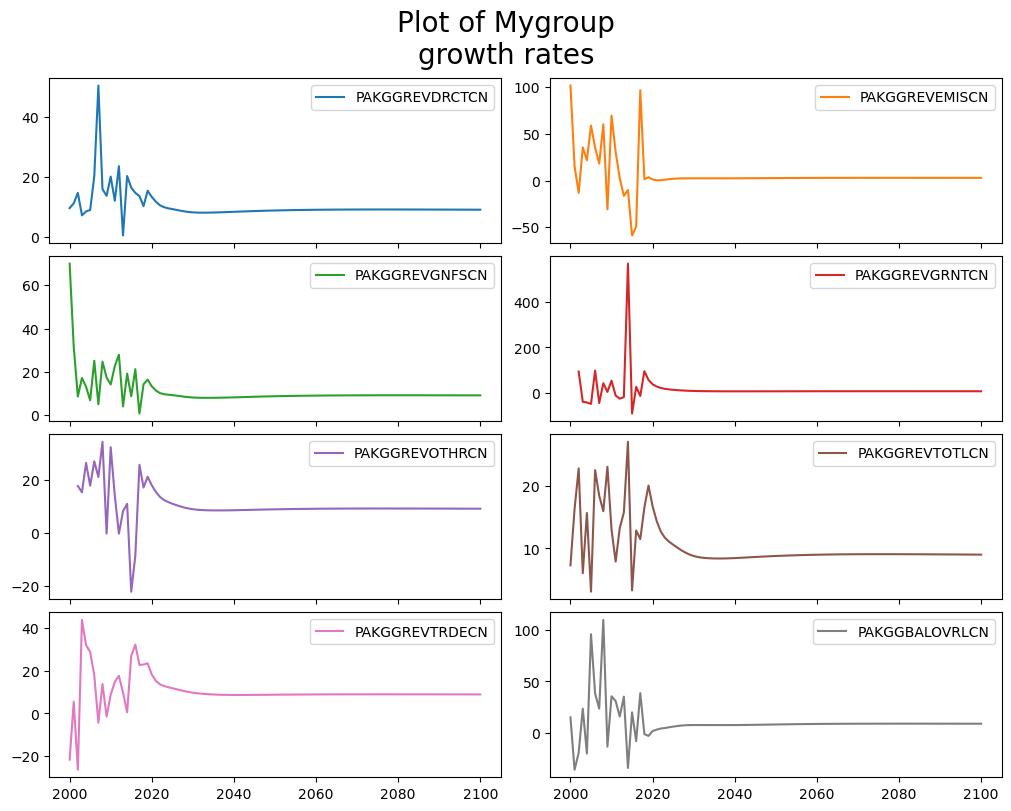
2.3.3. Display data from a group graphically#

mpak['#MyGroup'].pct.plot(title="Plot of Mygroup\ngrowth rates");

../../_images/0f1247e504325ee92252522ac48729bdb0a6093bd5dc7453fa6a8daf3ef1c5a5.png

2.4. Information about equations#

Information about specific equations can also be extracted and displayed.

2.4.1. The `endogene` property#

The endogene property returns a list of all variables in the model that are endogenous (have an equation). It can also be used to test whether a specific mnemonic has an equation associated with it.

The endogene property returns a list. For brevity only the first 5 elements are show below.

sorted(mpak.endogene)[:5]

['CHNEXR05', 'CHNPCEXN05', 'DEUEXR05', 'DEUPCEXN05', 'FRAEXR05']

The expression 'PAKNECONPRVTKN' in mpak.endogene returns True if the passed mnemonic is in the list returned by mpak.endogene.

'PAKNECONPRVTKN' in mpak.endogene

True

2.4.2. Retrieving info on equations#

There are three functions to extract the equations from a model.

Command	Effect
`mpak['PAKNECONPRVTKN'].frml`	Returns a normalized version of the equation (the one actually used in ModelFlow)
`mpak['PAKNECONPRVTKN'].eviews`	In models imported from Eviews, reports the original eviews specification
`mpak.PAKNECONPRVTXN.show`	Displays the equation (formula); variable descriptions; and variable values.

2.4.3. The `.eviews` method#

The mpak['PAKNECONPRVTKN'].eviews command returns the equations before they were normalized. In most cases this is a slightly more legible form. Here following the EViews syntax, \(\Delta ln()\) is written as dlog().

mpak['PAKNECONPRVTKN'].eviews

PAKNECONPRVTKN : 
DLOG(PAKNECONPRVTKN) =- 0.2*(LOG(PAKNECONPRVTKN( - 1)) - LOG(1.21203101101442) - LOG((((PAKBXFSTREMTCD( - 1) - PAKBMFSTREMTCD( - 1))*PAKPANUSATLS( - 1)) + PAKGGEXPTRNSCN( - 1) + PAKNYYWBTOTLCN( - 1)*(1 - PAKGGREVDRCTXN( - 1)/100))/PAKNECONPRVTXN( - 1))) + 0.763938860758873*DLOG((((PAKBXFSTREMTCD - PAKBMFSTREMTCD)*PAKPANUSATLS) + PAKGGEXPTRNSCN + PAKNYYWBTOTLCN*(1 - PAKGGREVDRCTXN/100))/PAKNECONPRVTXN) - 0.0634474791568939*@DURING("2009") - 0.3*(PAKFMLBLPOLYXN/100 - DLOG(PAKNECONPRVTXN))

2.4.4. The `.frml` property#

The .frml method returns the normalized equation that is actually used in ModelFlow.

In this instance the variable to be displayed is referenced directly (not as the result of a search operation ['partial*variablename'] syntax.

In addition to the equation of the variable, The .frml method also returns a long-text description of all the variables in the equation (assuming that one was defined for each variable), followed by a listing of all the dependent variables of the equation and their descriptions (below, the DURING_2019 variable has had no description defined so it returns a blank).

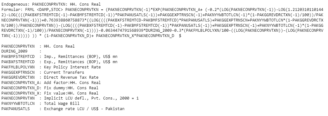
mpak.PAKNECONPRVTKN.frml

Endogeneous: PAKNECONPRVTKN: HH. Cons Real
Formular: FRML <DAMP,STOC> PAKNECONPRVTKN = (PAKNECONPRVTKN(-1)*EXP(PAKNECONPRVTKN_A+ (-0.2*(LOG(PAKNECONPRVTKN(-1))-LOG(1.21203101101442)-LOG((((PAKBXFSTREMTCD(-1)-PAKBMFSTREMTCD(-1))*PAKPANUSATLS(-1))+PAKGGEXPTRNSCN(-1)+PAKNYYWBTOTLCN(-1)*(1-PAKGGREVDRCTXN(-1)/100))/PAKNECONPRVTXN(-1)))+0.763938860758873*((LOG((((PAKBXFSTREMTCD-PAKBMFSTREMTCD)*PAKPANUSATLS)+PAKGGEXPTRNSCN+PAKNYYWBTOTLCN*(1-PAKGGREVDRCTXN/100))/PAKNECONPRVTXN))-(LOG((((PAKBXFSTREMTCD(-1)-PAKBMFSTREMTCD(-1))*PAKPANUSATLS(-1))+PAKGGEXPTRNSCN(-1)+PAKNYYWBTOTLCN(-1)*(1-PAKGGREVDRCTXN(-1)/100))/PAKNECONPRVTXN(-1))))-0.0634474791568939*DURING_2009-0.3*(PAKFMLBLPOLYXN/100-((LOG(PAKNECONPRVTXN))-(LOG(PAKNECONPRVTXN(-1)))))) )) * (1-PAKNECONPRVTKN_D)+ PAKNECONPRVTKN_X*PAKNECONPRVTKN_D  $

PAKNECONPRVTKN  : HH. Cons Real
DURING_2009     : 
PAKBMFSTREMTCD  : Imp., Remittances (BOP), US$ mn
PAKBXFSTREMTCD  : Exp., Remittances (BOP), US$ mn
PAKFMLBLPOLYXN  : Key Policy Interest Rate
PAKGGEXPTRNSCN  : Current Transfers
PAKGGREVDRCTXN  : Direct Revenue Tax Rate
PAKNECONPRVTKN_A: Add factor:HH. Cons Real
PAKNECONPRVTKN_D: Fix dummy:HH. Cons Real
PAKNECONPRVTKN_X: Fix value:HH. Cons Real
PAKNECONPRVTXN  : Implicit LCU defl., Pvt. Cons., 2000 = 1
PAKNYYWBTOTLCN  : Total Wage Bill
PAKPANUSATLS    : Exchange rate LCU / US$ - Pakistan

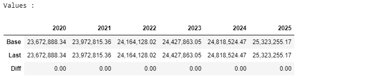
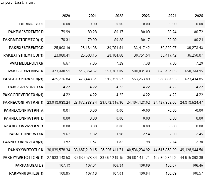
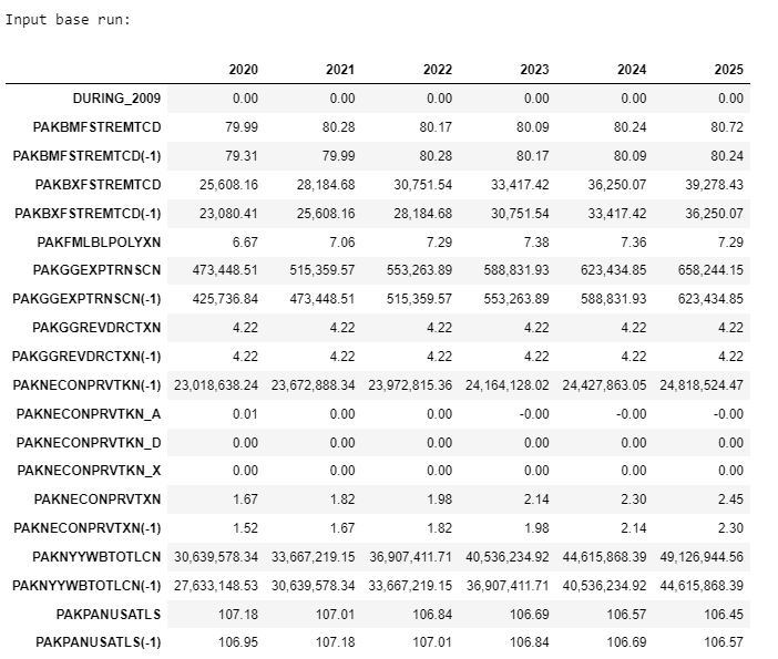
2.4.5. The `.show` method#

The .show method returns:

The description of the variable
The normalized equation that is actually used in ModelFlow.
A listing of the mnemonics and descriptions of the RHS variables
The data of that variable (drawn from the basedf and .lastdf DataFrames in the model object as well as the data of the RHS variables of the equation from both the basedf and .lastdf DataFrames.

mpak.smpl(2020,2025) #change the actual sample range to limit the number of columns displayed
mpak.PAKNECONPRVTKN.show

Working with a World Bank Model under ModelFlow

Contents

2. Working with a World Bank Model under ModelFlow#

2.1. Prepare the work space#

2.2. Load the model: Load a pre-existing model, data and descriptions#

2.2.1. The .modelload() method#

2.2.2. Extracting information about the model#

2.2.3. Information about variables#

2.2.3.1. The ! operator – searching on the variable description#

2.3. Groups#

2.3.1. The # operator – searching on the variable description#

2.3.2. Information about the data of series in a group#

2.3.3. Display data from a group graphically#

2.4. Information about equations#

2.4.1. The endogene property#

2.4.2. Retrieving info on equations#

2.4.3. The .eviews method#

2.4.4. The .frml property#

2.4.5. The .show method#

2.2.1. The `.modelload()` method#

2.2.3.1. The `!` operator – searching on the variable description#

2.3.1. The `#` operator – searching on the variable description#

2.4.1. The `endogene` property#

2.4.3. The `.eviews` method#

2.4.4. The `.frml` property#

2.4.5. The `.show` method#