6. A simulation that targets a specific outcome

Normally, when working with a model, the trajectory of the exogenous variables determine the trajectory of the endogenous (left hand side) variables. However, sometimes it can be useful to reverse the causality in the model, to find a trajectory for some exogenous variables that will result in certain endogenous variables achieving specific values.

A simple example might be where a policy maker wants to know what level of Carbon Tax, if implemented in a budget neutral fashion, would be needed to achieve a specific level of emissions. As specified, the analytical question is to achieve two targets:

1. A specific \(CO^2\) emissions trajectory

2. An unchanged fiscal deficit

In this Chapter - Targeting Specific Outcomes

This chapter illustrates how to target specific outcomes using ModelFlow. In the example, a specific outcome for carbon emissions is introduced and instruments (carbon taxes) are specified for achieving the target.

The chapter introduces a ModelFlow routine that searches for the values of the instruments (the carbon tax) that achieve the desired target level of carbon emissions (the target).

A second example illustrates a scenario with two targets (one a specific trajectory for emissions as above) and the second the stipulation that the policy be introduced in a budget neutral manner (a second target of an unchanged budget deficit) to be achieved by re-cycling Carbon tax revenues as transfers (a second instrument) to households.

In addition to these examples, techniques for fine-tuning the process in instances where the default parametrization of the system fails to find a result are also presented.

6.1. Targeting in ModelFlow

Targeting in ModelFlow requires that there be at least as many instruments as there are targets. So in the above example two instruments would be required.

The instrument to achieve the emissions could be a Carbon tax (applied uniformly on emissions from coal, gas and crude oil). The instrument to achieve an unchanged fiscal deficit, could be government spending or some form of revenue, say taxes on labor.

To illustrate targeting, the climate-aware model of Pakistan (Burns et al. [2021]) is used.

To run a targeting solution, the following main steps must be undertaken

1. Initialize a ModelFlow python session.

2. Load the model and data

3. Create a baseline

4. Define instrument variables (one instrument can consist of several variables).

5. Define a dataframe with the trajectory of the target variables.

6. Solve the problem using the .invert method.

7. Visualize the results

6.2. Load a model, data and descriptions

Following the initialization of the python session, the model is loaded and a model object mpak declared. The file pak.pcim contains the model object for the Pakistan model described in Burns (2021), including all of the equations data and variables.

mpak,initial = model.modelload('../models/pak.pcim')

Zipped file read:  ..\models\pak.pcim

mpak.var_description = mpak.var_description | {
    'PAKCCEMISCO2TKN' : 'Pakistan Total Carbon emissions (tons)'

} 

6.3. Solve the model to create a baseline

Next the model is solved, using the initial dataframe that was generated on the modelload.

In this instance, the model is solved from 2022 through 2100. The option ljit=True tells the model object to compile the model. Model compilation takes time, but once a model is compiled it will solve faster. When a model will be solved multiple times, the additional time required to compile the model, can be made up by the faster execution time each time the model is solved. Targeting requires the model to be solved many times, which makes the additional overhead of compilation worthwhile.

baseline = mpak(initial,2022,2100,alfa=0.7,silent=1,ljit=True)
mpak.basedf = baseline.copy()

Box 6. Compilation of a model

Python is an interpreted language, so solving can be improved by compiling the solving routines to machine code. The Numba package can help overcome this by translating Python code into machine code, significantly speeding up computation. The extent of this speed improvement depends on the complexity of the model and the computational resources required.

When solving a model, you can enable Numba compilation with by setting the option ljit=True

This setting cause the model to be compiled. The first time it is used for a model, the compilation will take some time. The compiled code is cached in the modelsource subfolder. As a result, subsequent runs of the model — even across different Python sessions — will use the precompiled model and solve much faster than the uncompiled versions.

Note: If there are issues with the solution, error messages may not be visible when the model is compiled. To troubleshoot, set ljit to False and rerun the model.

If you recreate a model with different logic but retain the same model name, consider clearing the modelsource subfolder to remove any cached compiled code that could interfere with the new model version.

6.4. Target CO2 emission - a very simple example

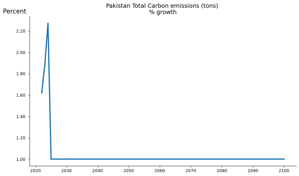
To illustrate the process for solving the model in targeting mode, an initial very simple example is set up, where only emissions are targeted (one target), and the objective is to have emissions grow at an annual rate of 1 percent.

6.4.1. Define targets

Having loaded the model, created a baseline and designated the target (steps 1-3 from above), the next step is to create the target variable(s).

This is done below by defining two series. The first, target_before_simple, is set equal to the value of the total emissions variable PAKCCEMISCO2TKN in the baseline. The second, target_simple, is the target for the same variable.

For this example we assume policy makers are looking for a carbon price that will restrict emissions growth to 1 percent per annum. The target_simple variable is therefore set equal to target_before_simple through 2024 and then, using the .upd() method, grown slowly at 1 percent per year afterwards.

# Create dataframe with only the target variable (for memmory)
target_before_simple = baseline.loc[2024:2100,['PAKCCEMISCO2TKN']]    

# create a target as a copy of the before variable through 2024 and then 
# having it grow by 1 percent per annum from 2025 onwards. 
target_simple = target_before_simple.upd(f'<2025 2100> PAKCCEMISCO2TKN =growth 1')

6.4.2. Define instruments

As noted above, for each target there must be one instrument. However, one instrument can consist of several instrument variables . Below the instrument is defined as three instrument variables: the carbon tax rate on each of Oil, Natural Gas and Coal. A list instruments_simple is created comprised of the mnemonics of each of the three variables.The three variables together are considered one instrument.

instruments_simple = [['PAKGGREVCO2CER','PAKGGREVCO2GER', 'PAKGGREVCO2OER']]

6.4.3. Finding the values for the instruments that achieve the desired target

To find the value for the instrument(s) that achieves the target of a 1 percent growth in emissions, the ModelFlow .invert() method is used: passing it the baseline database, the target dataframe that we defined above and the list of the instruments to use.

The .invert() method will solve the model once for each of the 77 years of the active sample period, and will solve multiple times for each year until it finds a set of instrument values that result in the desired targets. The dataframe containing the solution to the targeting problem is returned by the .invert() method and also stored in the .lastdf internal dataframe.

6.4.3.1. Invert options

The .invert() method has many options. The first three define the problem, the remainder influence how the solver operates. Finding the right options for a given problem is not always straightforward. The following table provides some hints on how to work with these options to optimize solution speed for a given problem.

Option	Parameters	Explanation
databank	name of dataframe	Dictates the initial conditions of the model (same as in a normal solve)
targets	list	A list of the variables to be targeted
instruments	list	A list of the variables that will be used as instruments to achieve the targets. Individual instruments may have multiple variables (as in the example above). Instrument list may contain Impulse parameters specific to the instrument (see below).
silent	bool	True: Suppress detailed outputs; False: Show detailed outputs (one line per iteration per year)
defaultimpuls	float	Determines the size of the change in instruments as the model searches for answers. Choose a value relative to the size of the actual series being modified.
defaultconv	float	Specifies the amount by which targeted variables may deviate from the target value and still be considered a solution. Should reflect the size of the target.
delay	Integer	Causes the instrument value changed to be lagged N periods from the target period being solved; For WBG models this should almost always be 0
varimpulse	bool	True: Sets the initial change in the instrument for the future to the same as in the most recently solved period. This will greatly speed solves where instruments are expected to evolve smoothly.
nonlin	integer	N: Jacobian will be updated after N iterations without a solution; Most WBG models are near-linear so setting to 0 will solve faster. If the solution fails, try non-linear=5
maxiter	integer	Maximum number of Newton iterations; If passed model will fail with a non-convergence error. If model does not converge try with nonlin=False
progressbar	boolean	default=False Determines whether or not a progress bar is displayed

6.4.3.2. Multiple instruments for one target

As mentioned, while there must be at least one instrument for each target it is possible to have more than one variable in a given instrument. Moreover, it is possible to assign specific impulse defaults to different instruments, or different weights for different variables in a multi-variable instrument.

Below are specific illustrations of how the instrument list can be specified.

Type	Instruments	Explanation
Single Target; Single Instrument	[‘myvar’]	The instrument list includes only one variable, default impulse
3 Targets; 3 Instruments, each with 1 variable	[‘myvar1’, ‘myvar2’, ‘Myvar3’]	All variables get the default impulse
2 Targets; 2 Instruments; different impulse	[(‘myvar1’,0.7), (‘myvar2’,.2000) ]	The first instrument takes an impulse value of 0.7 (presumably because its values are relatively small). The second takes a much larger impulse value of 2000, reflecting its larger scale.
2 Targets; 2 variables for first instrument; 1 for second	[[‘myvar1’, ‘myvar2’], ‘myvar3’)]	The first instrument takes two variables: myvar1 and myvar2; the second instrument has just one variable: myvar3
1 Target; 1 Instrument with 3 variables; different impulse	[[(‘myvar1’,50), (‘myvar2’,25), (‘myvar3’,10) ]]	Three instrument variables, each is assigned an impulse/weight, such that in finding values to achieve the target, ‘myvar’ will be pertubed twice as much as myvar2 and 5 times as much as myvar3
1 Target; 1 Instruments with 3 variables; smaller impulse	[(‘myvar1’,0.5), (‘myvar2’,0.25), (‘myvar3’,0.10)]]	Again three instrument variables, each is assigned an impulse/weight, such that in finding values to achieve the target, ‘myvar1’ will be perturbed twice as much as myvar2 and 5 times as much as MyVar3. NB this example will generate the same results as above, because although the impulse values have changed, the relative size of the impulse are the same

Note

The final section of this chapter explains in more detail the solution algorithm of the .invert() method and the meaning of the various options of the method.

6.4.4. Solving for the instruments to reach the targets

Below is the actual call to invert used for this example.

simple = mpak.invert(baseline,      # Invert calls the target instrument device                   
                targets = target_simple,                   
                instruments=instruments_simple,
                #invert options
                defaultimpuls=20,    # The default impulse instrument variables 
                defaultconv=2000.0,  # Convergergence criteria for targets
                varimpulse=True,     # Changes in instruments in each iteration 
                                     # are carried over to future iteratons
                nonlin=3,            # If no convergence after 3 iteration 
                                     # recalculate jacobian matrix 
                silent=True,         # Don't show iteration output 
                                     # (try False to show the results)
                maxiter = 3000,
                progressbar = True)

6.4.5. Display result

Once the simulation is complete the results are, as usual, stored in the mpak model object in the .lastdf dataframe. Results can be inspected either by using tables or graphically.

Below the .plot() method with option datatype='growth'is used to compare the total emissions and the carbon taxes from the solution set and the initial baseline, first in growth rates, then as a percent deviation from baseline option datatype='difpctlevel'. The option base_last=True ensures that the results from the most recent simulation (the lastdf DataFrame are displayed along side those from the basedf DataFrame. If multiple series are specified each series will be dispayed on a separate figure.

mpak.plot('PAKCCEMISCO2TKN',
          datatype='growth',
          legend=True,
          base_last=True).show

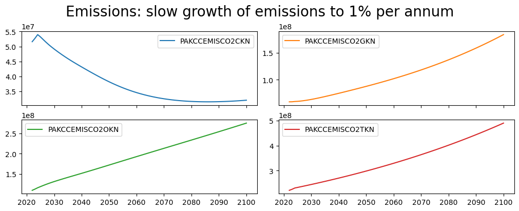
mpak['PAKCCEMISCO2?KN'].plot(
    title="Emissions: slow growth of emissions to 1% per annum",
    datatype='difpctlevel',
    showfig=True);

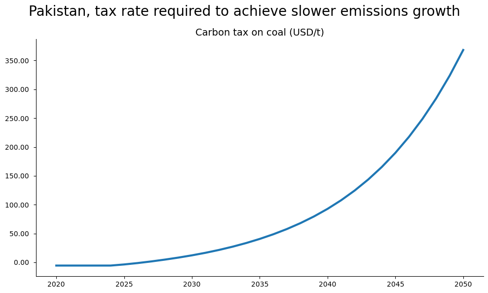
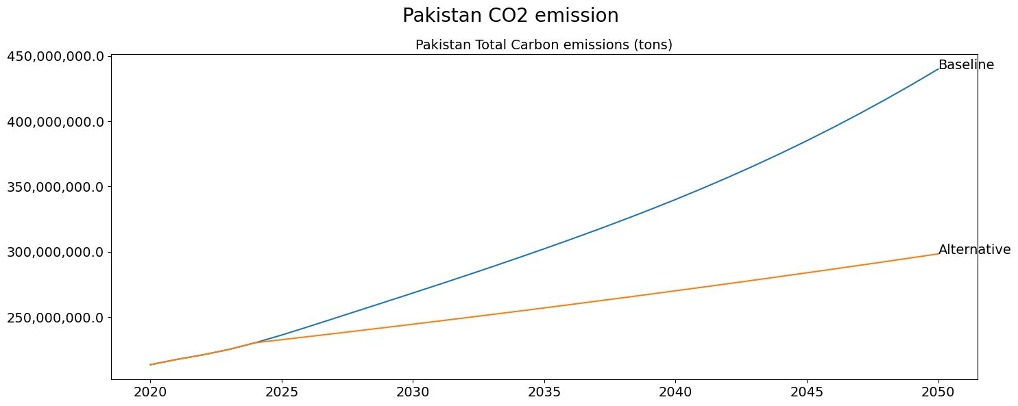
with mpak.set_smpl(2020,2050):    # change if you want another  timeframe 
    fig1=mpak.plot('PAKCCEMISCO2TKN',
          datatype='level',
          legend=True,
          base_last=True)
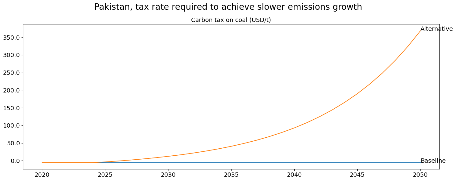
    fig2=mpak.plot('PAKGGREVCO2CER',
          datatype='level',
          title=f'Pakistan, tax rate required to achieve slower emissions growth',
                   base_last=True,
          legend=True)
combo=(fig2+fig1)
combo.show    

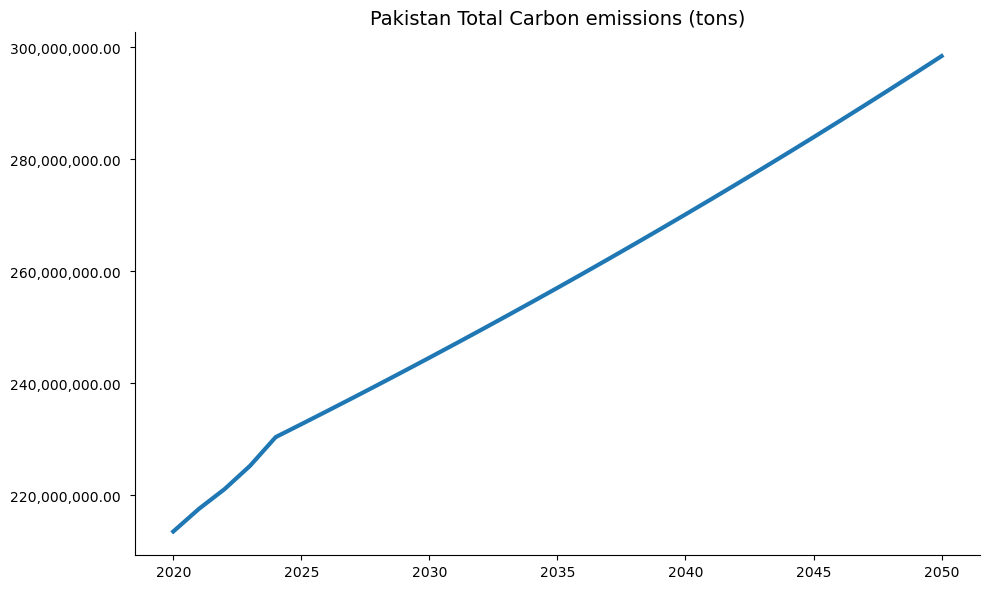
with mpak.set_smpl(2020,2050):    # change if you want another  timeframe 
    fig = mpak[f'PAKCCEMISCO2TKN'].plot_alt(title='Pakistan CO2 emission') 
    fig2 = mpak[f'PAKGGREVCO2CER'].plot_alt(
    title=f'Pakistan, tax rate required to achieve slower emissions growth'); 
    
fig1
fig2

6.5. Targeting carbon emissions in a budget neutral manner

In this example, a more complex targeting exercise is conducted.

In this instance two targets are identified:

1. An unchanged fiscal deficit

2. A 40 percent decline in overall emissions

This requires at least two instruments:

1. The carbon emissions target will be determined by 3 instrument variables (the carbon taxes on each of coal, oil and natural gas)

2. The fiscal balance target will be met by one instrument Government spending on goods and services, implying that revenues from the Carbon Taxes will be used to increase government services.

Burns et al.(2021), using the same model explores, the macroeconomic consequences implications of alternative uses of the revenues from the Carbon Tax.

Note

there is no technical restriction on what instruments to choose, However,if instruments are chosen that have little influence on the targets, ModelFlow is unlikely to find values for the instruments that achieve the desired levels of the target variables.

6.5.1. Define target trajectory for CO2 emission.

The objective is to reduce Carbon emissions by 40% (as compared with the baseline) by the year 2050 and hold them constant in level terms afterwards.

The two variables reduction_percent, which reflects by how much emissions are to decline, and achieved_by, which represents by when the reduction should be achieved, are used to define the objectives series in a flexible way.

Using variables like this to express the constraint may be a bit more complicated. However, in the long run it may be easier as it allows the same code to be used to explore how different emission targets and different years in which the target should be fulfilled might affect the results.

reduction_percent = 40  # Input the desired reduction in percent. 
achieved_by       = 2050

If the target is to achieve a 40 percent reduction in emissions by 2050, the pathway toward that objective can be described as a rate of growth of emissions that leads us to a 40 percent lower level by 2050.

That growth rate can be calculated by:

1. Calculating the level of emissions to be reached in the target year as \(PAKCCEMISCO2TKN_{2050} \cdot (1-40/100)\)

2. Calculate the growth rate of the target variable needed to reach that level in 2050=
   \(\biggl(\dfrac{PAKCCEMISCO2TKN_{2050}\cdot (1-40/100)}{PAKCCEMISCO2TKN_{2024}}\biggr)^{\dfrac{1}{2050-2024}}-1\)

Once the target is defined the model can then calculate the values of carbon taxes necessary to reach those levels.

Below the target growth rate is calculated.

bau_emissions_final = baseline.loc[achieved_by,'PAKCCEMISCO2TKN'] #baseline emissions
                                                                  # in 2050
bau_emissions_2024  = baseline.loc[2024,'PAKCCEMISCO2TKN'] #baseline emissions 
                                                           # in 2024

target_emissions_final  = bau_emissions_final*(1-reduction_percent/100) #target
                                                               # emissions in 2050

#growth rate needed between 2024 and 2050 to reach the target emissioons level in 2050
target_growth_rate  = (target_emissions_final/bau_emissions_2024)**(1/(achieved_by-2024))-1
bau_growth_rate     = (bau_emissions_final/bau_emissions_2024)**(1/(achieved_by-2024))-1

Below a quick routine to display the parameters and objectives.

print(f"Baseline Emissions in {achieved_by}               : {bau_emissions_final:13,.0f} tons")
print(f"Target  Emissions  in {achieved_by}               : {target_emissions_final:13,.0f} tons")
print(f"Business as usual growth rate in percent : {bau_growth_rate:13,.1%}")
print(f"Target growth rate in percent            : {target_growth_rate:13,.1%}")

Baseline Emissions in 2050               :   439,930,561 tons
Target  Emissions  in 2050               :   263,958,337 tons
Business as usual growth rate in percent :          2.5%
Target growth rate in percent            :          0.5%

6.5.2. Create a dataframe with the target emissions

To prepare the simulation, a dataframe needs to be prepared with the target variable(s) set to the desired growth path, calculated above.

The target dataframe will contain as many variables as there are targets, at this stage just one.

Initially the target variable is set to the values of the original data in the baseline, then it is set to grow at the growth rate calculated above between 2024 and 2050 to achieve the 40 percent reduction in emissions and then it is held constant at this level.

# Create dataframe with only the target variable (data defined from 2024 onwards)
target_before = baseline.loc[2024:,['PAKCCEMISCO2TKN']]     
# create a target dataframe with a projection of the target variable 
target = target_before.upd(f'<2025 {achieved_by}> PAKCCEMISCO2TKN =growth {100*target_growth_rate}')
target = target.upd(f'<{min(2100,achieved_by+1)} {2100}> PAKCCEMISCO2TKN = {target_emissions_final}')
#target.loc[:2055]

6.5.3. Create target for government deficit

In this example, there is a second target – to maintain the government deficit unchanged. As the objective is to hold the deficit constant as a share of GDP (at the levels in the baseline), the target for this variable will just take the same values as the government balance variable (expressed as a percent of GDP) PAKGGBALOVRLCN_ in the baseline.

#add to the target dataframe the GG balance variable from 2022 through 2100
target.loc[:,'PAKGGBALOVRLCN_'] = baseline.loc[2022:2100,'PAKGGBALOVRLCN_']

The target dataframe now holds two Series, defined over the period 2024 through 2100.

target

	PAKCCEMISCO2TKN	PAKGGBALOVRLCN_
2024	2.303703e+08	-3.131896
2025	2.315794e+08	-3.045253
2026	2.327948e+08	-2.984815
2027	2.340166e+08	-2.945600
2028	2.352449e+08	-2.921505
...	...	...
2096	2.639583e+08	-2.540508
2097	2.639583e+08	-2.540567
2098	2.639583e+08	-2.540636
2099	2.639583e+08	-2.540713
2100	2.639583e+08	-2.540798

77 rows × 2 columns

6.6. Define instruments

The instruments to achieve these targets are the 3 carbon taxes and government spending on goods and services. To find the mnemonics for these variables a search is done over the descriptions of the variables, first over the carbon tax:

mpak['!*Carbon*'].des

PAKCCEMISCO2TKN : Pakistan Total Carbon emissions (tons)
PAKGGREVCO2CER  : Carbon tax on coal (USD/t)
PAKGGREVCO2GER  : Carbon tax on gas (USD/t)
PAKGGREVCO2OER  : Carbon tax on oil (USD/t)

A separate search is done to identify the government spending variable to be used as an instrument. It makes sense to use a variable which has a fairly direct impact on the government deficit.

mpak['!*government*expenditure*goods*'].des

PAKGGEXPGNFSCN        : General government expenditure on goods and services (millions lcu)
PAKGGEXPGNFSCN_A      : Add factor:General government expenditure on goods and services (millions lcu)
PAKGGEXPGNFSCN_D      : Fix dummy:General government expenditure on goods and services (millions lcu)
PAKGGEXPGNFSCN_FITTED : Fitted  value:General government expenditure on goods and services (millions lcu)
PAKGGEXPGNFSCN_X      : Fix value:General government expenditure on goods and services (millions lcu)

For the purposes of this simulation the PAKGGEXPGNFSCN_A variable (the add-factor for the government spending on goods and services equation) is selected. The add-factor is chosen so that the underlying equation remains active during the simulation.

Then a list called instruments is populated with two lists:

• the first is a list of variables for the first instrument (in this case the three carbon taxes)

• the second a list of one instruments for the second instrument (just one variable the add-factor on government spending on goods and services

instruments = [['PAKGGREVCO2CER','PAKGGREVCO2GER', 'PAKGGREVCO2OER'],
               'PAKGGEXPGNFSCN_A']   

6.7. Solve the two-target targeting problem:

Having defined the dataframes for the target values and the instrument variables, the model can be solved.

Note

The %%times command at the beginning of the cell below instructs Jupyter Notebook to keep track of how long it takes for the cell to execute and displays the result.

%%time  
unweighted= mpak.invert(baseline,          # Invert calls the targeting routine 
                targets = target.loc[:,: ],#our targets defined above           
                instruments=instruments,   # our instruments defined above
                defaultimpuls=20,          # The default impulse value for the instruments 
                defaultconv=2000.0,        # Convergergence criteria for targets ( a relatively large number)
                varimpulse=True,           # Change in instruments after each iteration are carried over to the future
                nonlin=5,                  # If no convergence in 15 iteration recalculate jacobi 
                silent=True,               # Don't show iteration output 
                delay=False,
                maxiter = 75,
                progressbar = True)

CPU times: total: 9.06 s
Wall time: 9.13 s

6.7.1. Results

The following two chart illustrate that the objective of slowing emissions growth was achieved, with the growth rate in the targeted series equal to 1 percent.

mpak.plot('PAKCCEMISCO2TKN',base_last=True,legend=False).show

Below the carbon tax that was required to achieve the desired emissions result.

with mpak.set_smpl(2020,2050):
    mpak['PAKGGREVCO2CER'].plot_alt(title='Carbon tax on coal: baseline versus target ')

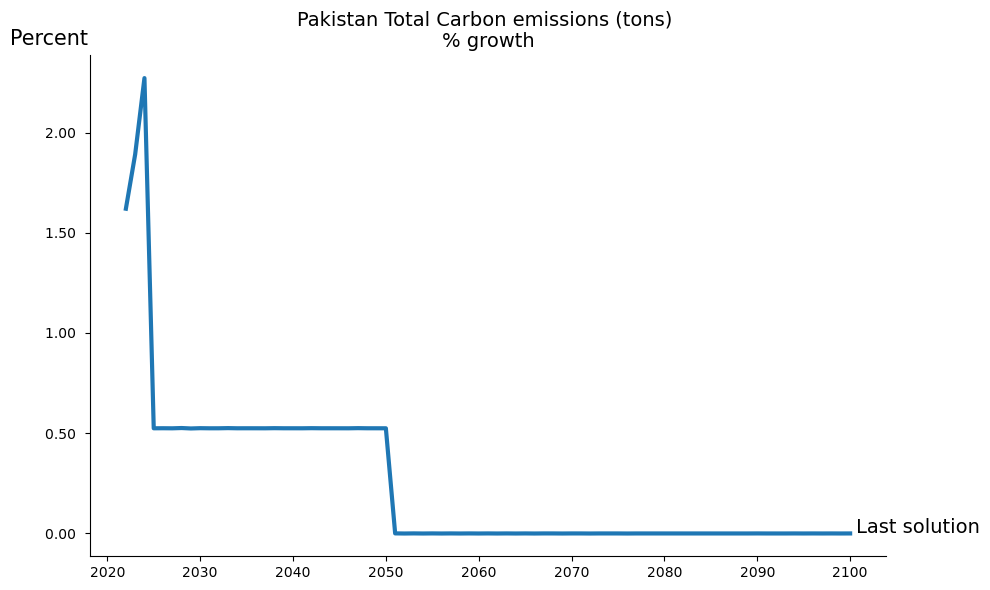
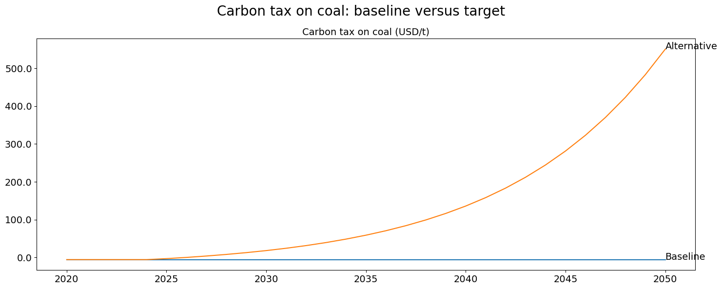
fig2.figs.keys() 

dict_keys(['Pakistan Total Carbon emissions (tons), growth'])

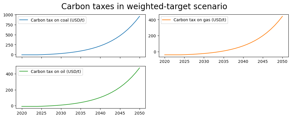
6.8. Weighting the instruments

When using multiple instruments for a single target, the modeler may want to privilege changes in one instrument over another by specifying weights to attach to each. In the example below, specific weights are attached to the instruments, instructing the solver to place twice as much emphasis on adjusting the carbon tax on coal emissions (as compared with the other two carbon taxes). The actual number applied to the weights is not important as it is the relative weights that play a role. Thus here the weights 50,25,25 would have precisely the same effect as 2,1,1.

new_instruments =[[('PAKGGREVCO2CER',50),
                   ('PAKGGREVCO2GER', 25),
                   ('PAKGGREVCO2OER',25)],
                 'PAKGGEXPGNFSCN_A']

weighted = mpak.invert(baseline,    # Invert calls the target instrument device                   
                targets = target.loc[:,: ],                   
                instruments=new_instruments,
                defaultimpuls=20, # The default impulse instrument variables 
                defaultconv=2000.0,  # Convergergence criteria for targets
                varimpulse=True,  # Changes in instruments in each iteration are carried over to the future
                nonlin=5,     # If no convergence in 15 iteration recalculate jacobi 
                silent=True,        # Don't show iteration output 
                delay=0,
                maxiter = 50,
                progressbar = True)

With a weight twice as large on the coal carbon tax instrument, the carbon tax on coal rises to a level twice as fast as that of the other carbon taxes.

with mpak.set_smpl(2020,2050):    # change if you want another  timeframe 
    fig1 = mpak[f'PAKGGREVCO2CER PAKGGREVCO2GER PAKGGREVCO2OER' ].rename().plot(
        title='Carbon taxes in weighted-target scenario ') 
    
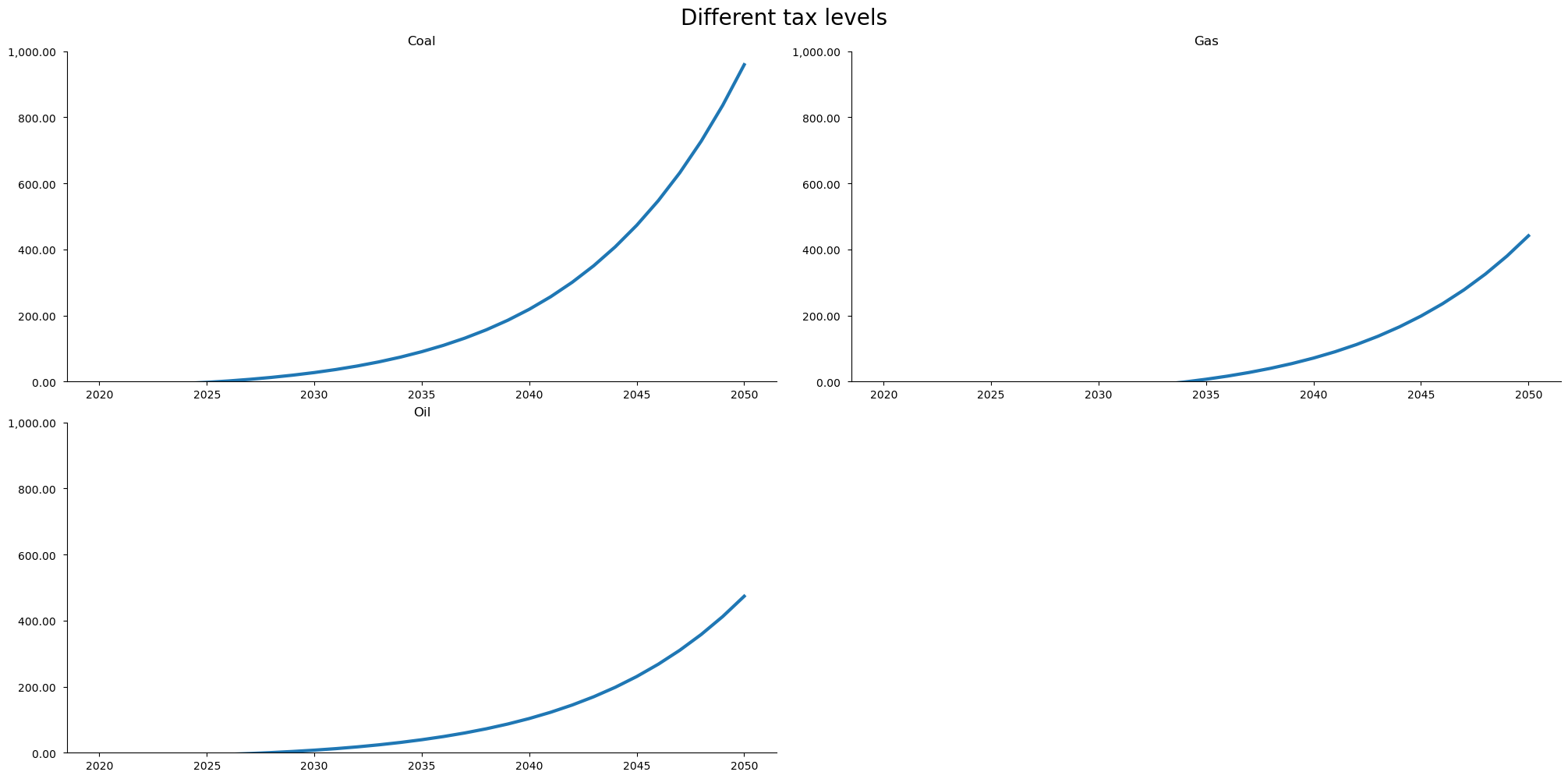
with mpak.set_smpl(2020,2050):    # change if you want another  timeframe 
    fig = mpak.plot('PAKGGREVCO2CER PAKGGREVCO2GER PAKGGREVCO2OER',
                   datatype='level',base_last=True,name='fignewstyle',
                   mul=1,samefig=True,title='Different tax levels')    
fig.figs['fignewstyle'].axes[0].set_title('Coal')    
fig.figs['fignewstyle'].axes[1].set_title('Gas')    
fig.figs['fignewstyle'].axes[2].set_title('Oil')  
fig.figs['fignewstyle'].axes[0].set_ylim(0, 1000)
fig.figs['fignewstyle'].axes[1].set_ylim(0, 1000)
fig.figs['fignewstyle'].axes[2].set_ylim(0, 1000)
fig.show       

Instead of putting different weights on the carbon taxes, an alternative might have been to add more instruments to the budget balance target (say direct and indirect taxes), with the weights equal to each tax type’s share in total revenues. Set up this way, the scenario would maintain budget balance neutrality by using the revenues from the carbon taxes to reduce other (perhaps more distorting taxes).

Box 7. Targeting background

The concept of targets and instruments in economic modeling was introduced by Tinbergen [1967]

When solving a targeting problem it can be thought as follows:

Take a generic system of equations (a model): \(\textbf{y}_t= \textbf{F}(\textbf{x}_{t})\)

Where, \(\textbf{x}_{t}\) are all predetermined variables - lagged endogenous and exogenous variables.

A condensed model (\(\textbf{G}\)) can be defined comprised of a few endogenous variables (\(\bar{\textbf{y}}_t\)) – the targets and a few a few exogenous variables(\(\bar{\textbf{x}}_{t}\)) – the instrument variables.

In this model, the remaining predetermined variables are fixed. Thus this model can be expressed as \(\bar{\textbf{y}}_t= \textbf{G}(\bar{\textbf{x}}_{t})\).

In some models the result depends on the level of exogenous variables with a lag. For instance in a disease spreading model, the number of infected on a day depends on the probability of transmission some days before. If the probability of transmission is the instrument and the number of infected is the target. Therefor it can be useful to allow a delay, when finding the instruments. In this case we want to look at \(\textbf{y}_t= \textbf{F}(\textbf{x}_{t-delay})\)

Inverting G, gives a model where instruments are a functions of targets: \(\bar{\textbf{x}_{t-delay}}= \textbf{G}^{-1}(\bar{\textbf{y}_{t}})\).

In other words, the inverted model is solved for the value of the instruments that gives the desired level for the targets: \(\textbf{G}^{-1}(\bar{\textbf{y}_{t}})\)

For most models \(\bar{\textbf{x}}_{t-delay}= \textbf{G}^{-1}(\bar{\textbf{y}_{t}})\) does not have a nicely closed-form solution. However it can be solved numerically – in ModelFlow this is done using the Newton–Raphson method.

So \(\bar{\textbf{x}}_{t-delay}= \textbf{G}^{-1}(\bar{\textbf{y}_{t}^*})\) will be found using :

for \(k\) = 1 to convergence

\(\bar{\textbf{x}}_{t-delay,end}^k= \bar{\textbf{x}}_{t-delay,end}^{k-1}+ \textbf{J}^{-1}_t \times (\bar{\textbf{y}_{t}^*}- \bar{\textbf{y}_{t}}^{k-1})\)

\(\bar{\textbf{y}}_t^{k}= \textbf{G}(\bar{\textbf{x}}_{t-delay}^{k})\)

convergence: \(\mid\bar{\textbf{y}_{t}^*}- \bar{\textbf{y}_{t}} \mid\leq \epsilon\)

ModelFlow uses numerical differentiation, to find the Jacobian of the inverted matrix because it is simple and fast.

\(\textbf{J}_t = \frac{\partial \textbf{G} }{\partial \bar{\textbf{x}}_{t-delay}}\)

\(\textbf{J}_t \approx \frac{\Delta \textbf{G} }{\Delta \bar{\textbf{x}}_{t-delay}}\)

Mechanically that requires the model should be solved once for each instrument with a given delta applied to the targets. Recording the impact on each of the targets from the \({\Delta {x}_{t-delay}^{instrument}}\) gives and estimate of \(\textbf{J}_t\)

In order for \(\textbf{J}_t\) to be invertible there has to be the same number of targets and instruments.

However, each instrument can be a basket of exogenous variable an they can have different impulse \(\Delta\) .

(6.1)\[\begin{equation} \Delta x^{instrument=i} = \begin{bmatrix} \Delta x^{instrument=i,variable=1} \\ \Delta x^{instrument=i,variable=2} \\ \Delta x^{instrument=i,variable=3} \\ \vdots \\ \Delta x^{instrument=i,variable=n} \\ \end{bmatrix} \end{equation}\]

When an instrument changes the variables will change and the change will be in the proportions defined by their impulse.

Notice that the level of \(\bar{\textbf{x}}\) is updated (by \(\textbf{J}^{-1}_t \times (\bar{\textbf{y}_{t}^*}- \bar{\textbf{y}_{t}}^{k-1})\)) in all periods from \(t-delay\) to \(end\), where \(end\) is the last timeframe in the dataframe. This is useful for many applications, where the instruments are level variable (i.e. not change variables).

This is the default behavior. It can be changed.

6.9. Tuning the target input to get a result

Models implemented in ModelFlow can be very different, and the targeting routine .invert() is fairly general. In many cases, targeting will not work out-of-the-box, its options will have to be tweaked to fit the problem at hand.

6.9.1. Targetting options

The invert options that affect the speed and accuracy of a solution are:

• defaultimpuls

• defaultconv

• nonlin

• maxiter

• varimpulse

6.9.2. defaultimpuls – set the size of the delta used when calculating the Jacobian

The impulse variable determines the size of the delta that is used to calculate the jacobian matrix. If it is too small or too large the resulting jacobian will solve only very slowly. Typically the impulse should be scaled in relation to the magnitude of the instrument it is to impact.

If a large impulse is used for a small variable (or a small impulse for a large variable) \(\textbf{x}+{\Delta \bar{\textbf{x}}_{t-delay}}\) the model may become unsolvable.

Separate impulse values can be set for each instrument. This is done when setting the instruments (see discussion below).

6.9.3. nonlin – an integer - set to the number of iterations to attempt before recalculating the Jacobian

If the model is nonlinear it makes sense to re-estimate the jacobian matrix \(\textbf{J}_t\) frequently. The nonlin=a number option allows the user to set the number of iterations the solver should allow without finding a solution before calculating a new jacobian.

If:

• nonlin=0 the jacobian will not be updated (default) – implicitly indicates the model should be treated as if linear.

• nonlin=<a number> the same jacobi matrix will be updated after <a number> iterations. -nonlin=3, 5 and 10 are all reasonable options in cases where model non-linearity requires the recalculation of he Jacobian.

6.9.4. Convergence

The targeting is stopped when all target variables converge. The convergence criteria should reflect the size of the target variables. Too large and the solution may not actually reflect a close approximation of the target, too small and the model may take a very long-time to solve.

• defaultconv=<a number>

6.9.5. Maximum number of iterations

• maxiter=<a number>

This option determines the maximum number of iterations that the model should run in trying to find a solution. Reasonable initial numbers may be between 50 and 100. If a model takes more than 100 iterations, there may be an issue. Potentially the chosen instruments do not have much impact on the target variables, or the model is relatively non-linear. Try setting nonlin=10 to see if recalculating the Jacobian allows the model to solve.

6.10. Definition of Instruments

As noted above there must be at least one instrument for each target. Instruments are passed as a python list.

Each element in the list is an instrument.

• An element can be:

  • a variable name

  • a tuple with a variable name and an associated impulse \(\Delta\)

  • an inner list which defines which contains:

    • a list of variable names. Each element in the inner list is an instrument variable

    • a list of tuples each tuple contains a variable name and the associated impulse \(\Delta\).

The \(\Delta\) variable(s) is (are) used in the numerical differentiation. Also if one instrument contains several variables, the proportion of each variable will be determined by the relative \(\Delta variable\).