1. Model structure and causal chains#
A model has a well defined logical and causal structure. Kogiku(1968) provides an introduction to causal analysis of models, while Berndsen(1995) gives a more elaborate discussion.
At the simplest level, the equations of a model can be organized into blocks.
Simultaneous block include equations that have are co-determined simultaneously. They contain feedback loops that may require several iterations before a solution that satisfies them all is found. A classic simultaneous block would include GDP, Income and Consumption. Consumption depends on income. Income depends on GDP, but Consumption also determines GDP.
Recursive blocks include equations that are a simple function of other variables. For example, the current account balance is just the difference between Export Revenues and Import Revenues. These can be solved with just one pass once the values of the simultaneous blocks have been resolved.
At the equation level, each endogenous variable is a function of one or more variables, but because some of these variables are also dependent on other variables in the model, those right hand side variables that are endogenous can have their equations substituted into the first level equation to get an extended set of dependencies. Moreover, the endogenous right hand side variables of these second level variables can also have their right hand sides substituted into the equation etc.
ModelFlow uses the networkx python package to analyze the interrelationships within the model and between equations and includes a number of methods and properties to present these interrelationships both in tabular and graphical form [1], a subset of which is exposed in this chapter.
1.1. Setting up the python environment and loading a pre-existing model#
In this chapter - Model struicture and causal chains
This chapter introduces tools and techniques for analyzing the structure and behavior of models in the ModelFlow framework. In a system of equations like World Bank models, impacts on variables in a simulation can be the results of the direct effect from changes imposed on variables in the equation of a variable, but also indirect effects caused by changes in variables that are not in the equation of a specific variable, but do generate changes in variables that are in the equation.
The chapter presents tools that explore the structure of a model, and display both the direct and indirect determinants of given equations.
Following a simulation, the routines presented can display the precise contribution of a given variable to the change in another.
In addition to displaying which variables impacted a given variable, the routines can also be used to understand which variables are most impacted by changes in a given variable.
Results can be displayed both graphically and in tabular form.
mpak,baseline = model.modelload('../models/pak.pcim',alfa=0.7,run=1)

mpak.model_description="World Bank climate aware model of Pakistan as described in Burns et al. (2019)"
Zipped file read: ..\models\pak.pcim
latex=True # Enables the charts in latex
Note
latex=True
The default behavior when displaying graphs in a jupyter notebook is to produce images in .svg format. These images scale well and the mouseover feature can be used. That is: On mouseover of a node, the variable and the equation are displayed. On mouseover on a joining line, the extent to which the variable contributed to the change in the dependent variable is displayed.
Unfortunately this jupyter book (book – not notebook) requires images be in the jpg or PNG format. To enable generation of PDFs the latex=True option is set, which forces ModelFlow routines to render graphics in the PNG format – effectively disabling the features of svg.
If using the Notebooks that for this book, the variable latex could be set equal to False in which case the same code will generate graphics in the more versatile SVG format.
1.2. Model information#
As noted before, the model object contains information about the model itself, its name, its structure (does it contain simultaneous equations or is it recursive), the number of variables it contains and the number that are exogenous and endogenous (have associated equations).
mpak
<
Model name                              :                  PAK
Model structure                         :         Simultaneous
Number of variables                     :                  839
Number of exogeneous  variables         :                  461
Number of endogeneous variables         :                  378
>
1.3. Model structure#
A quick way to visualize the structure of a model is to plot its adjacency matrix (https://en.wikipedia.org/wiki/Adjacency_matrix).
The adjacency matrix plots the relationships between endogenous variables in the model, dividing them into one or more simultaneous blocks and one or more recursive blocks.
Below is the adjacency matrix for the Pakistan model. Variables in the red square block (simultaneous block) depend on one or more variables that in turn depend upon them, requiring the model to solve for their values simultaneously. The variables in the green triangles (recursive blocks) do not enter directly or indirectly as an argument in the variables that determine them and therefore can be solved in one iteration once the values for the simultaneous variables are determined.
Internally ModelFlow takes these factors into consideration and solves the simultanrous block(s) first and then solves the recursive blocks.
mpak.plotadjacency(size=(20,20));
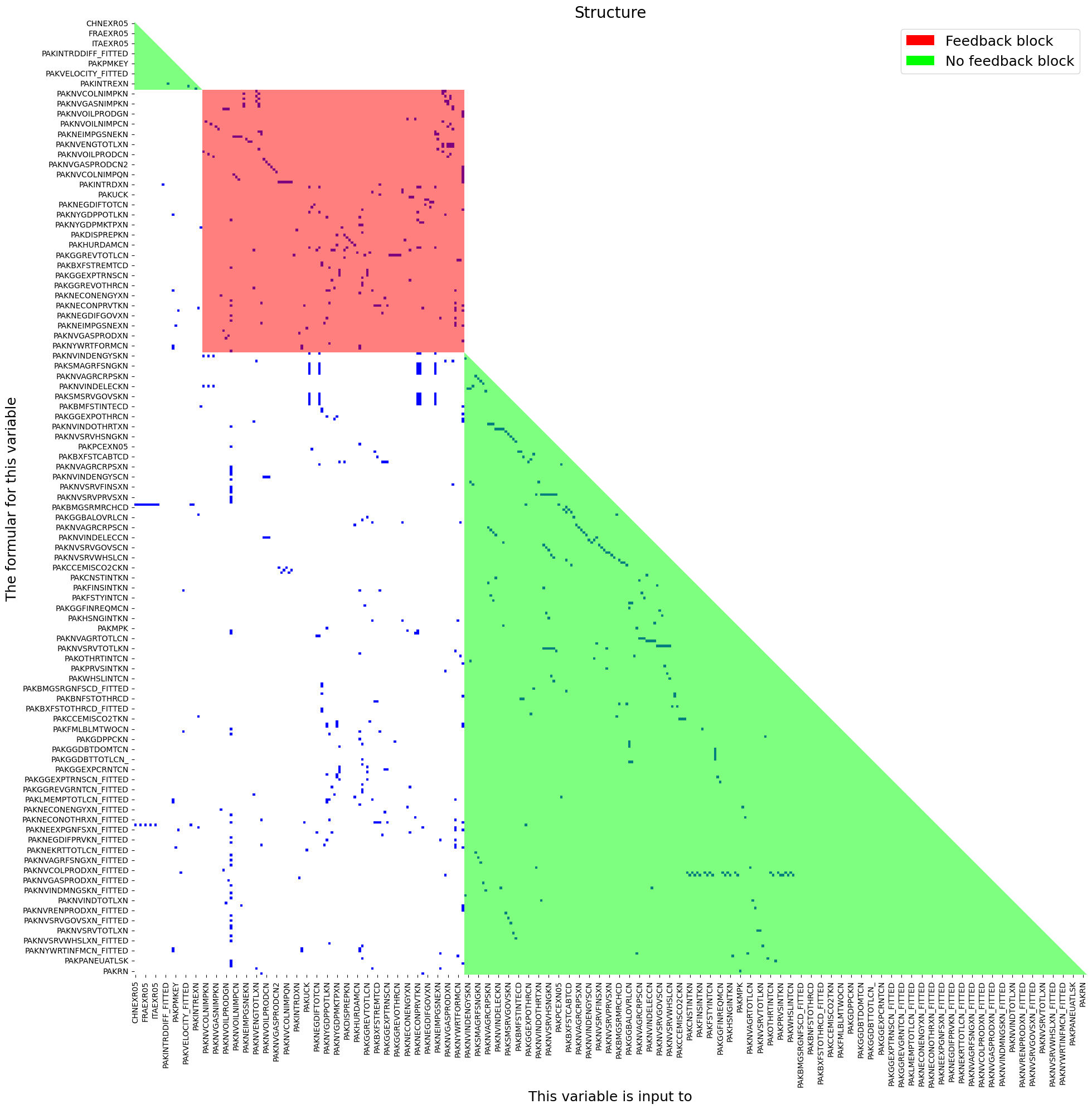
As is evident in the above chart, the majority of the variables in MFMod Pakistan are recursive (green) and depend simply on the values of other variables. The core of the model lies in the simultaneous (red) block, where the main wages, prices, real and nominal variables that drive other variables are determined.
1.4. The dependencies of individual endogenous variables (the .tracepre() method)#
As noted above, every endogenous variables is directly dependent on the variables that occur on its right hand side, but is also indirectly dependent on the variables that determine its RHS variables and in turn those that determine the variables to the right of them ad infinitum.
ModelFlow includes several methods and properties that allow these dependencies to be explored.
The .frml property returns the normalized formula of an equation, from which the right hand variables for the equation can be discerned and these are reported along with their descriptions following the formula.
mpak.PAKNECONPRVTKN.frml
Endogeneous: PAKNECONPRVTKN: HH. Cons Real
Formular: FRML <DAMP,STOC> PAKNECONPRVTKN = (PAKNECONPRVTKN(-1)*EXP(PAKNECONPRVTKN_A+ (-0.2*(LOG(PAKNECONPRVTKN(-1))-LOG(1.21203101101442)-LOG((((PAKBXFSTREMTCD(-1)-PAKBMFSTREMTCD(-1))*PAKPANUSATLS(-1))+PAKGGEXPTRNSCN(-1)+PAKNYYWBTOTLCN(-1)*(1-PAKGGREVDRCTXN(-1)/100))/PAKNECONPRVTXN(-1)))+0.763938860758873*((LOG((((PAKBXFSTREMTCD-PAKBMFSTREMTCD)*PAKPANUSATLS)+PAKGGEXPTRNSCN+PAKNYYWBTOTLCN*(1-PAKGGREVDRCTXN/100))/PAKNECONPRVTXN))-(LOG((((PAKBXFSTREMTCD(-1)-PAKBMFSTREMTCD(-1))*PAKPANUSATLS(-1))+PAKGGEXPTRNSCN(-1)+PAKNYYWBTOTLCN(-1)*(1-PAKGGREVDRCTXN(-1)/100))/PAKNECONPRVTXN(-1))))-0.0634474791568939*DURING_2009-0.3*(PAKFMLBLPOLYXN/100-((LOG(PAKNECONPRVTXN))-(LOG(PAKNECONPRVTXN(-1)))))) )) * (1-PAKNECONPRVTKN_D)+ PAKNECONPRVTKN_X*PAKNECONPRVTKN_D  $

PAKNECONPRVTKN  : HH. Cons Real
DURING_2009     :
PAKBMFSTREMTCD  : Imp., Remittances (BOP), US$ mn
PAKBXFSTREMTCD  : Exp., Remittances (BOP), US$ mn
PAKFMLBLPOLYXN  : Key Policy Interest Rate
PAKGGEXPTRNSCN  : Current Transfers
PAKGGREVDRCTXN  : Direct Revenue Tax Rate
PAKNECONPRVTKN_A: Add factor:HH. Cons Real
PAKNECONPRVTKN_D: Fix dummy:HH. Cons Real
PAKNECONPRVTKN_X: Fix value:HH. Cons Real
PAKNECONPRVTXN  : Implicit LCU defl., Pvt. Cons., 2000 = 1
PAKNYYWBTOTLCN  : Total Wage Bill
PAKPANUSATLS    : Exchange rate LCU / US$ - Pakistan
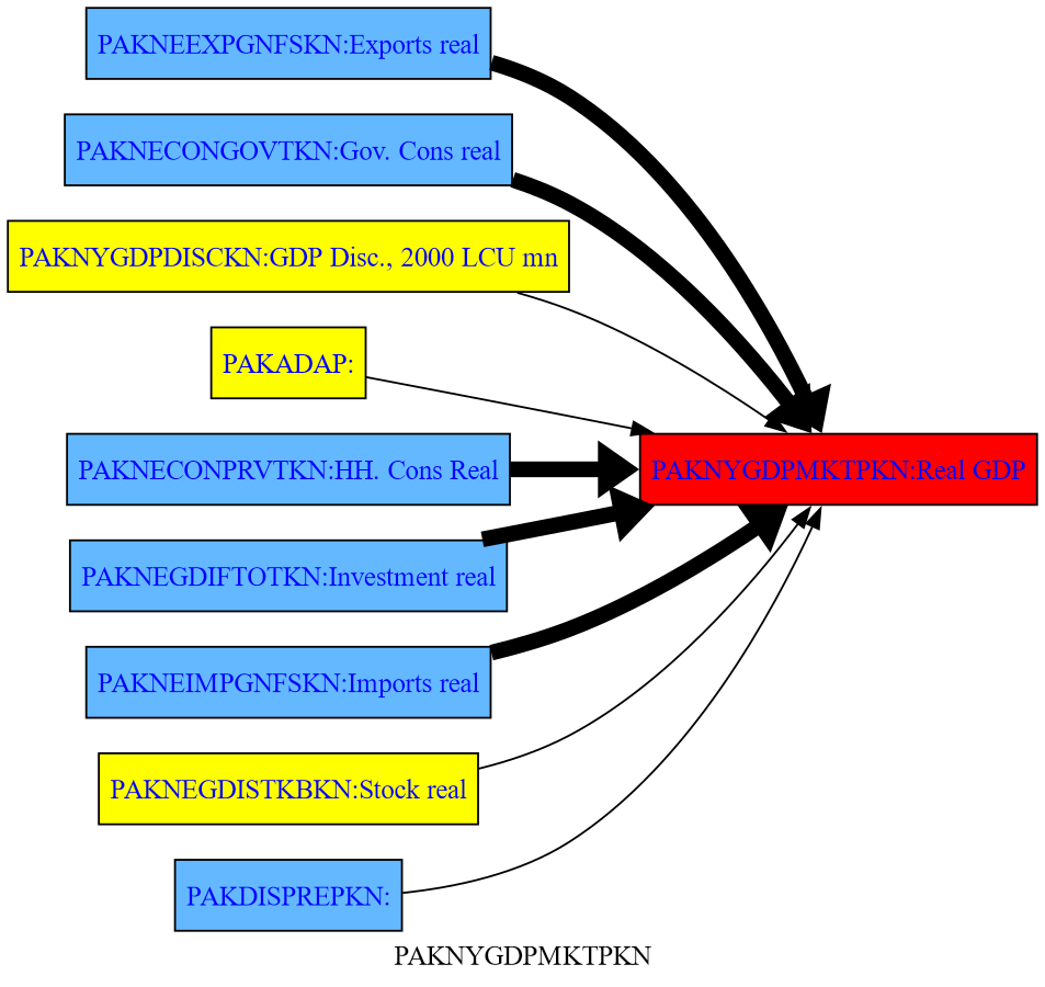
The method .tracepre() provides a graphical representation of this relationship, showing all the variables that directly determine an endogenous variable (in this example real GDP), distinguishing between RHS variables that are endogenous (in blue) and those that are exogenous (yellow).
mpak.PAKNYGDPMKTPKN.tracepre(png=latex,size=(4,3))
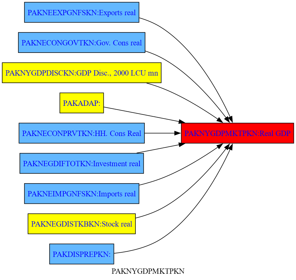
If the model has been solved, .tracepre() goes one step further and uses the thickness of the lines to reflect the relative importance of each variable in the change of the dependent variable in the preceding scenario.
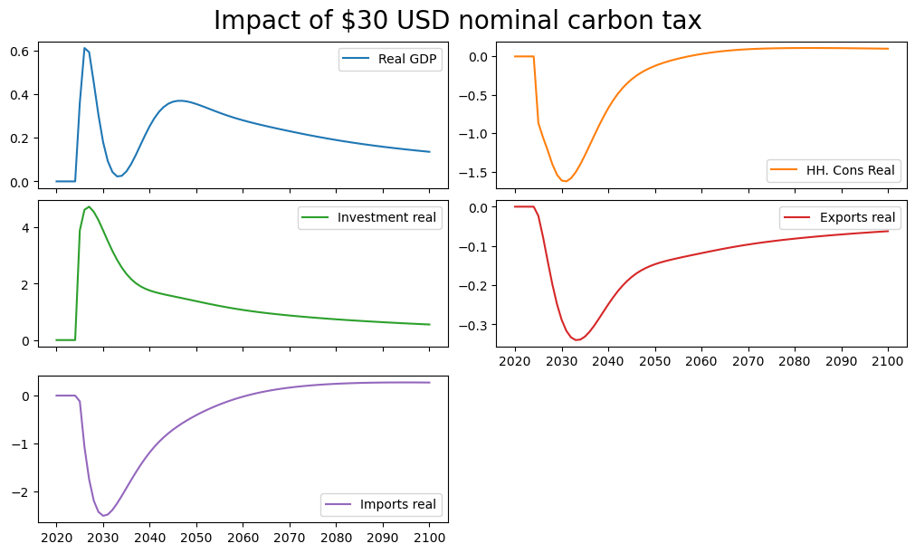
1.4.1. Shock the model#
Below a $30 nominal Carbon tax is applied beginning in 2025.
alternative  =  baseline.upd("<2025 2100> PAKGGREVCO2CER PAKGGREVCO2GER PAKGGREVCO2OER = 30")
result = mpak(alternative,2020,2100) # simulates the model
As a result GDP, consumption investment and most all variables in the model change, as illustrated in the below graphs that show the percent deviation of the main components of GDP from their baseline values.
mpak['PAKNYGDPMKTPKN PAKNECONPRVTKN PAKNEGDIFTOTKN PAKNEEXPGNFSKN PAKNEIMPGNFSKN'].difpctlevel.rename().plot(title="Impact of $30 USD nominal carbon tax");
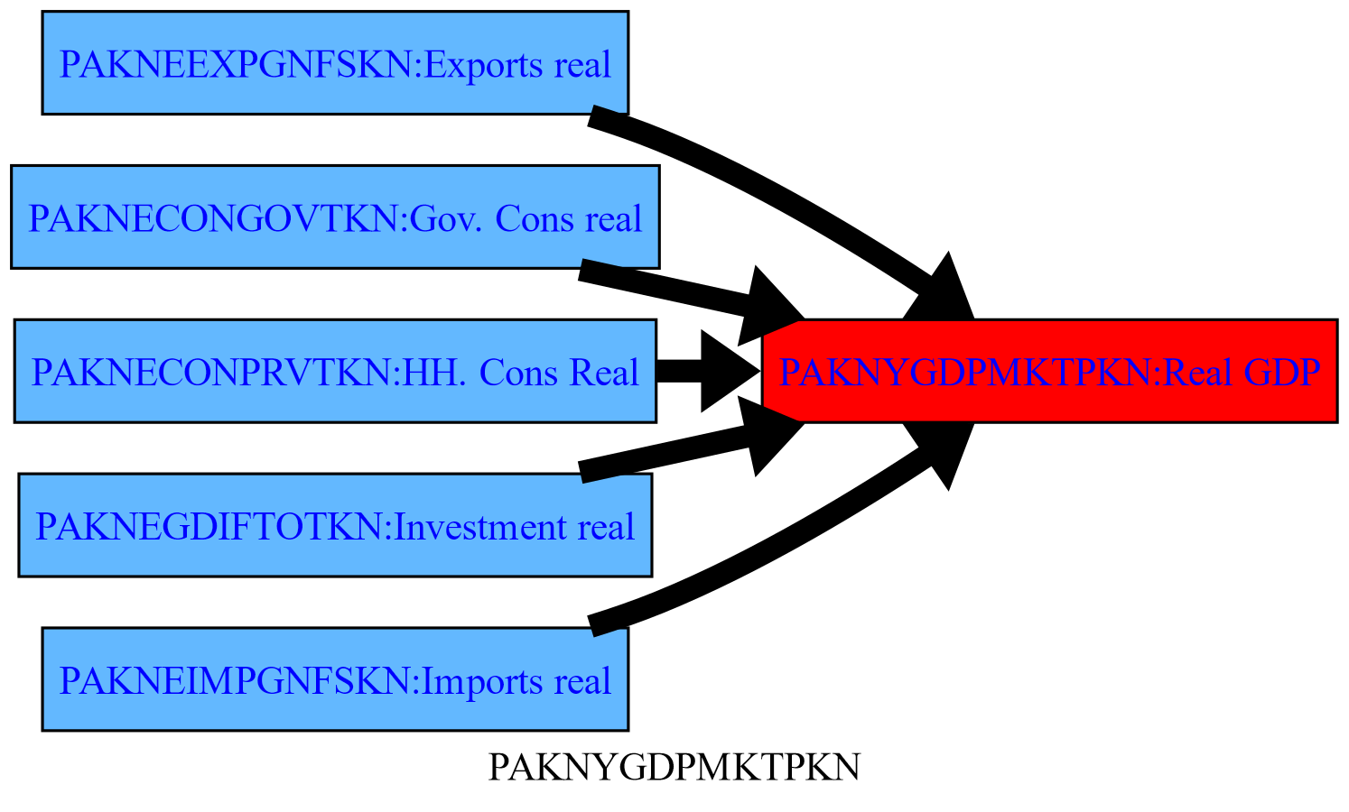
1.4.2. .tracepre() following a shock#
Below the same .tracepre() command is executed again, but because a shock has been simulated, the width of the lines representing the causal links between variables is thicker the more important the change in a given variable was in the previous simulation in explaining the change in the level of the dependent variable (GDP).
latex=True
mpak.PAKNYGDPMKTPKN.tracepre(png=latex,size=(5,3))
1.4.3. The filter option, restricts the output of .tracepre()#
The filter option can be used to restrict the output of .tracepre() to RHS variables that have had a large impact on the dependent variable. In the example below, the option filter=20 instructs tracepre to only draw those rhs variables that contributed 20 percent or more to the total change in GDP.
mpak.PAKNYGDPMKTPKN.tracepre(filter=20,png=latex,size=(5,3))
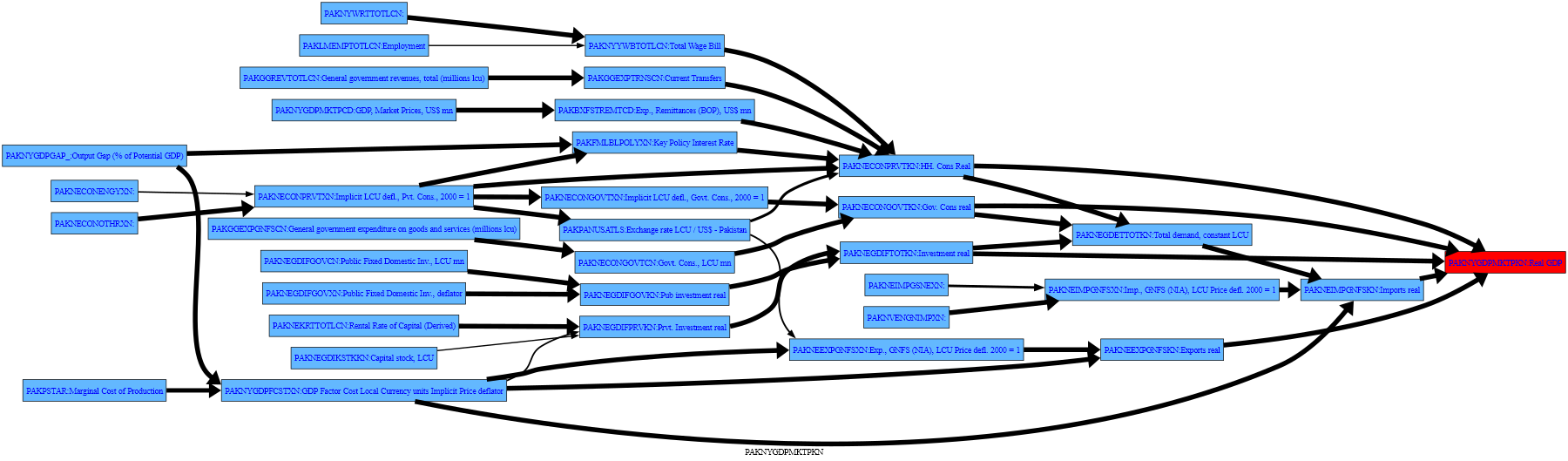
1.4.4. The up option, extends the .tracepre plot beyond the first level of causal variables#
The up option allows .tracepre dependencies to be followed beyond the first level of causal variables. Below, it is extended to variables as much as three levels back, and restricted to those whose variation explains at least 20 percent of the change in the variable of which they are a right-hand-side variable.
mpak.PAKNYGDPMKTPKN.tracepre(filter = 20,up=3,png=latex)
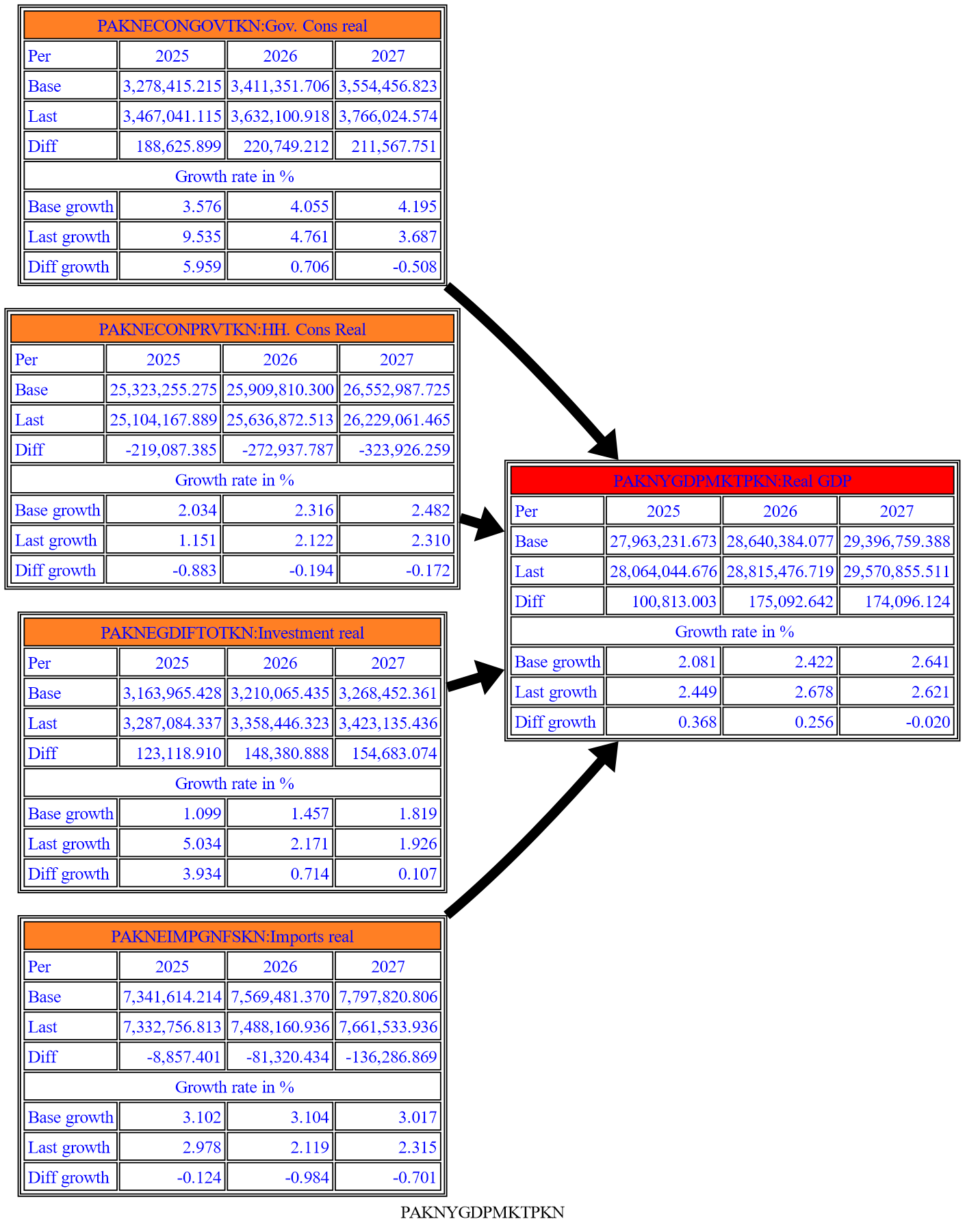
1.4.4.1. Adding a table to the causal graph#
The Fokus2 option causes a table of values to be added to the casual flow graph. In this example, the showgrowth=True option instructs ModelFlow to show the table in both level and growth rate terms.
with mpak.set_smpl(2025,2027):
    print(mpak.PAKNYGDPMKTPKN.tracepre(filter = 20,
                fokus2='PAKNEGDIFTOTKN PAKNECONPRVTKN PAKNECONGOVTKN PAKNYGDPMKTPKN PAKNEIMPGNFSKN',
                growthshow=True,
                png=latex)
         )
None
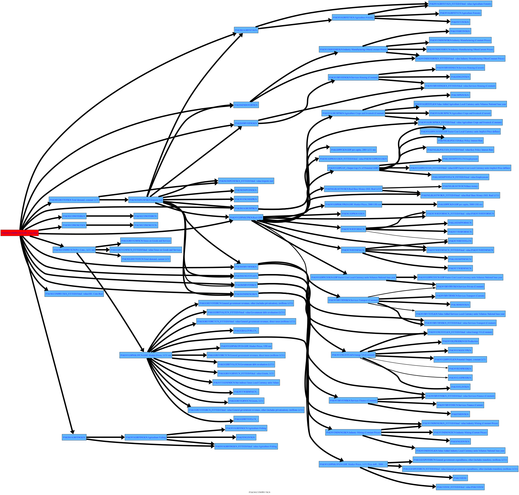
1.4.5. .tracedep(down=xx) traces the impact of a variable on other variables#
The preceding examples have focused on understanding how changes in other variables have impacted the variable of interest. The closely related tracedep() method shows what other variables depend on the specified variable, with the down=xx option indicating how many levels of substitution to display. Here, the direction of the dependency graph is reversed and the chart shows the impact that the changes in the selected variable had on those which depend upon it. Below is the impact of change in consumption on all of the variables up to 3 levels below the consumption equation.
mpak.PAKNECONPRVTKN.tracedep(down=3,filter=20,png=latex)
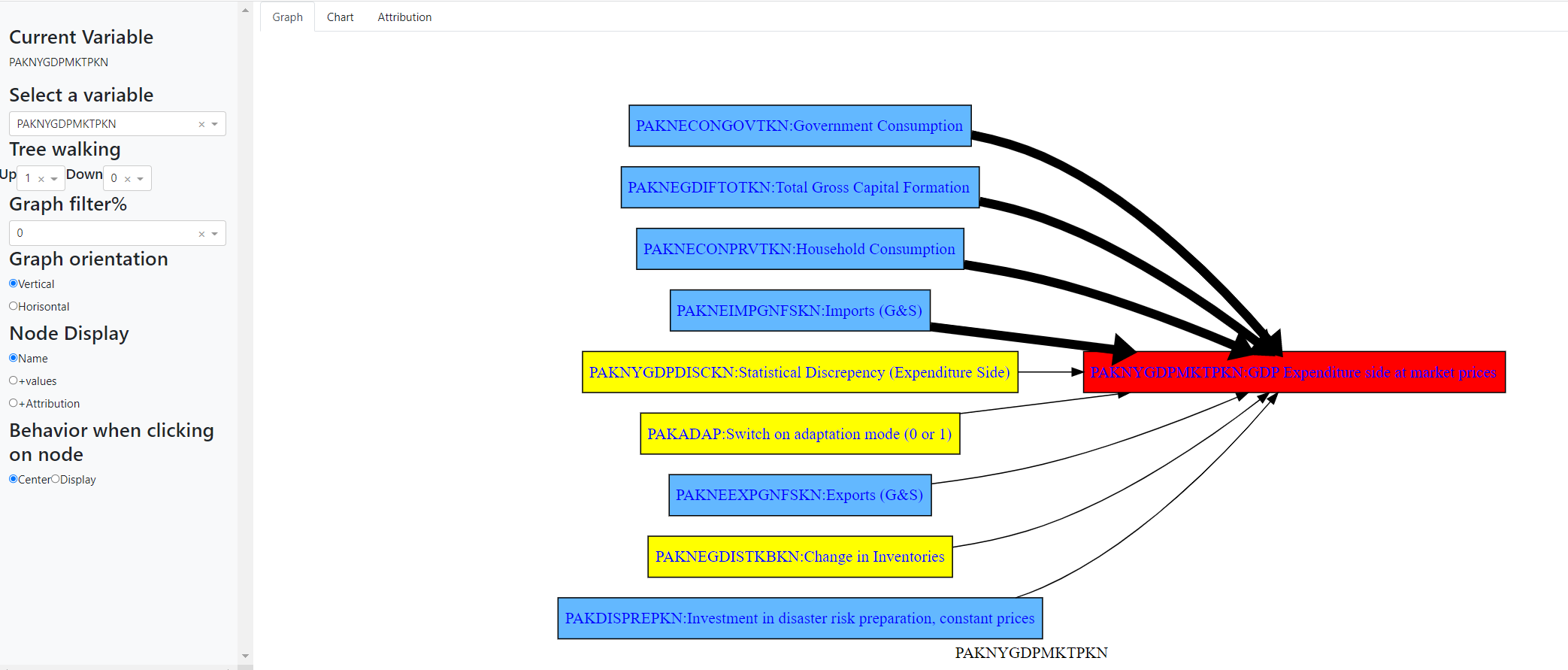
1.4.6. .modeldash() An interactive way to explore dependencies#
The .modeldash() method generates a widget that allows you to dynamicaly adjust the arguments to the tracepre() and tracedep functions.
 with mpak.set_smpl(2022,2026):
        mpak.modeldash('PAKNYGDPMKTPKN',jupyter=True,inline=False)
The above commands generate a dashboard that looks a like the below, where the panel to the left allows the user to change options including the filter, the depth of the trace among other things.