The .upd() method returns a DataFrame with updated variables.

1.4. The `.upd()` method returns a `DataFrame` with updated variables.#

The .upd() method extends pandas by giving the user a concise and expressive way to modify data in a DataFrame using a syntax that a database-manager or macroeconomic modeler might find more natural.

.upd() can be used to:

Perform different types of updates
Perform multiple updates each on a new line
Perform changes over specific periods
Use one input which is used for all time frames, or a separate input for each time
Preserve pre-shock growth rates for out of sample time-periods
Display results

Note

.upd() does not change the value of the DataFrame upon which it operates, but its results can be assigned to a DataFrame. In the examples below the originating DataFrame df is never overwritten. It could be, by assigning the result of an upd() command to df, i.e.

df.upd('B = 7')

would set B from the DataFrame df equal to 7 and the function returns a temporary DataFrame whose results can be visualized. The values of df are not changed in this example.

By contrast:

df=df.upd('B = 7')

performs the same operation but assigns the results of the operation to df – overwriting its earlier values.

Warning

The syntax of an update command requires that there be a space between variable names and the operators.

Thus df.upd("A = 7") is fine, but df.upd("A =7") will generate an error.

Similarly df.upd("A * 1.1") is fine, but df.upd("A* 1.1") will generate an error.

1.4.1. some examples of the `.upd()` method#

First, create a dataframe using standard pandas syntax. In this instance with years as the index and a dictionary defining the variables and their data.

# Create a dataframe using standard pandas

df = pd.DataFrame({'B': [1,1,1,1,1,1],'C':[1,2,3,6,8,9],'E':[4,4,4,4,4,4]},index=[v for v in range(2020,2026)])
                  
df

	B	C	E
2020	1	1	4
2021	1	2	4
2022	1	3	4
2023	1	6	4
2024	1	8	4
2025	1	9	4

1.4.1.1. Use `.upd` to create a new variable#

With standard pandas a user can add a column (series) to a DataFrame simply by assigning a value to an new column name (NEW2 had existed its values would have been updated. For example:

df['NEW2']=[17,12,14,15]

.upd() provides this functionality as well.

df.upd('c = 142.0')

	B	C	E
2020	1	142.0	4
2021	1	142.0	4
2022	1	142.0	4
2023	1	142.0	4
2024	1	142.0	4
2025	1	142.0	4

Note

The new variable name was entered as a lower case ‘c’ here. Lowercase letters are not legal ModelFlow variable names. The .upd() method knows that it is part of ModelFlow and knows this rule. As a result, it automatically translates lowercase entries into upper case so that the statement works.

The automatic creation of new variables can be suspended by setting the option: create = False. For more look see the discussion of the 'upd() option create=True.

1.4.2. Multiple updates and specific time periods#

The ModelFlow method .upd() takes a string as an argument. That string can contain a single update command or can contain multiple commands (for muliple lines the needs to be passed using triple apostrophes ''' or three quote symbols """ as below.

Moreover, by including a <Begin End> date clause in a given update command, the update will be restricted to the associated time period.

The below illustrates this, modifying two existing variables A, B over different time periods and creating two new variables, C and D.

Note

Inheritance of time periods in the .upd() method The third line inherits the time period of the previous line.

Note also, the submitted string can include comments as well (denoted with the standard python # indicator).

df.upd("""
# Same number of values as years
<2021 2024> A = 42 44 45 46    # 4 years
<2020     > B = 200            # 1 year 
c = 500                        # Same period as previous line
<-0 -1> D = 33                   # All years 
""")

	B	C	E	A	D
2020	200.0	500.0	4	0.0	33.0
2021	1.0	2.0	4	42.0	33.0
2022	1.0	3.0	4	44.0	33.0
2023	1.0	6.0	4	45.0	33.0
2024	1.0	8.0	4	46.0	33.0
2025	1.0	9.0	4	0.0	33.0

Note

The method .upd() only operates on one variable. A command like .upd('A = B') would not work. For these kind of functions, use .mfcalc() (see next section).

1.4.3. Update several variables in one line#

Sometime there is a need to update several variable with the same value over the same time frame. To ease this case .upd() can accept several left-hand side variables in one line

df.upd('''
<2022 2024> h i j k =      40      # earlier values are set to zero by default
<2020>      p q r s =       1000   # All values beginning in 2020 set to 1000
<2021 -1>   p q r s =growth 2      # -1 indicates the last year of dataframe
''')

	B	C	E	H	I	J	K	P	Q	R	S
2020	1	1	4	0.0	0.0	0.0	0.0	1000.000000	1000.000000	1000.000000	1000.000000
2021	1	2	4	0.0	0.0	0.0	0.0	1020.000000	1020.000000	1020.000000	1020.000000
2022	1	3	4	40.0	40.0	40.0	40.0	1040.400000	1040.400000	1040.400000	1040.400000
2023	1	6	4	40.0	40.0	40.0	40.0	1061.208000	1061.208000	1061.208000	1061.208000
2024	1	8	4	40.0	40.0	40.0	40.0	1082.432160	1082.432160	1082.432160	1082.432160
2025	1	9	4	0.0	0.0	0.0	0.0	1104.080803	1104.080803	1104.080803	1104.080803

Box 2. Time scope of .upd() commands

If the user wants to modify a series or group of series for only a specific point in time or a period of time, she can indicate the period in the command line.

If one date is specified the operation is applied to a single point in time
If two dates are specifies the operation is applied over a period of time.

The selected time period will persist until re-set with a new time specification. This is useful if several variables are going to be updated for the same time period, but must be kept in mind if subsequent commands are to operate over a different time period.

The time period can be reset to the full time-period by using the special <-0 -1> time period. More generally:

-0 indicates the start of the dataframe
-1 indicates the end of the dataframe

If no time is provided the dataframe start and end period will be used.

The = operator causes the left-hand side variable to be set equal to the values following the = operator.

Note

Either:

Only one data point is provided. In this case its value is applied to all dates in the indicated period, or
The number of data points provided must match the number of dates in the period specified.

In the example below:

The first line sets the variable A during the specified period to specific values
The second line sets the variable B to 200 in 2023
The third line inherits the time period set in the second line (2023) and sets the variable C equal to 500.

df.upd("""
# Same number of values as years
<2021 2024> A = 42 44 45 46    # 4 years
<2023     > B = 200            # 1 year 
c = 500                        # inherits previous time-period specification (2023)
""")

	B	C	E	A
2020	1.0	1.0	4	0.0
2021	1.0	2.0	4	42.0
2022	1.0	3.0	4	44.0
2023	200.0	500.0	4	45.0
2024	1.0	8.0	4	46.0
2025	1.0	9.0	4	0.0

1.4.4. Operators of the `.upd()` method#

The .upd() method takes a variety of mathematical operators, some of these are described below.

Types of update:

Update to perform	Use this operator
Set a variable equal to the input	=
Add the input to the LHS variable	+
Set the variable to itself multiplied by the input	*
Increase/Decrease the variable by a percent of itself - i.e. multiplies itself by (1+input/100)	%
Set the growth rate of the variable to the input	=growth
Change the growth rate of the variable to its current growth rate plus the input value	+growth
Set the amount by which the variable should increase from its previous period level (\(\Delta = var_t - var_{t-1}\))	=diff

1.4.4.1. The “=” operator: assign a value(s) to a variable#

With standard pandas a user can add a column (series) to a DataFrame simply by assigning a adding to a DataFrame. For example:

df['NEW2']=[11,17,12,14,15,17]

df.upd('NEW2 = 11 17 12 14 15 17') provides this functionality as well.

Note that with .upd() the multiple values are space delimited, versus standard pandas where they are passed as a comma delimited list.

df.upd('NEW2 = 11 17 12 14 15 17')

	B	C	E	NEW2
2020	1	1	4	11.0
2021	1	2	4	17.0
2022	1	3	4	12.0
2023	1	6	4	14.0
2024	1	8	4	15.0
2025	1	9	4	17.0

1.4.4.2. The “+” operator adds to the existing values in the specified range#

In the example below 42 is added to the pre-existing values of the variable B over the period 2022 and 2024, and a different value is subtracted from each of the three rows selected.

df.upd('''
# Or one number to all years in between start and end 
<2022 2024> B  +  42    # one value broadcast to 3 years 
<2022 2024> E  +  -1 -2 -3 # add (subtract) a different value to each of the three rows specified
''')

	B	C	E
2020	1.0	1	4.0
2021	1.0	2	4.0
2022	43.0	3	3.0
2023	43.0	6	2.0
2024	43.0	8	1.0
2025	1.0	9	4.0

1.4.4.3. The * operator multiplies all values in a range by the specified values#

In the example below the pre-existing values of the variable A for years 2021, 2022 and 2023 are multiplied by three different numbers (42, 44 and 45 respectively).

df.upd('''
# Same number of values as years
<2021 2023> B *  42 44 55
''')

	B	C	E
2020	1.0	1	4
2021	42.0	2	4
2022	44.0	3	4
2023	55.0	6	4
2024	1.0	8	4
2025	1.0	9	4

1.4.4.4. The % operator increases all values in a range by a specified percent amount#

In this example:

A new column is generated with value 1 in every year
A is increased by 42 and 44% over the range 2021 through 2022.
B is increased by 10 percent in all years
C The values of C are overwritten and set to 100 for the whole range (because the previous line set the active range to <-0 -1>)
C is decreased by 12 percent over the range 2023 through 2025.

df.upd('''
<-0 -1> A = 1
<2021 2022 > A %  42 44   # Two specific years / rows
<-0 -1> B % 10            # all rows 
C = 100                   # all rows persist 
<2023 2025> C % -12       # now only for 3 years 
''')

	B	C	E	A
2020	1.1	100.0	4	1.00
2021	1.1	100.0	4	1.42
2022	1.1	100.0	4	1.44
2023	1.1	88.0	4	1.00
2024	1.1	88.0	4	1.00
2025	1.1	88.0	4	1.00

1.4.4.5. The =GROWTH operator sets the percent growth rate to specified values#

The =GROWTH operator sets the growth rate of the variable to the indicated level.

res = df.upd('''
# Same number of values as years
<-0 -1> A = 100
<2021 2022> A =GROWTH  1 5  
<2020> c = 100 
<2021 2025> c =GROWTH 2 
''')
# print the resulting DataFrame (res) first as levels and then as a growth rate uising the pandas pct_change() method
print(f'Dataframe:\n{res}\n\nGrowth:\n{res.pct_change()*100.0}\n') 

Dataframe:
      B           C  E       A
1  100.000000  4  100.00
1  102.000000  4  101.00
1  104.040000  4  106.05
1  106.120800  4  100.00
1  108.243216  4  100.00
1  110.408080  4  100.00

Growth:
        B    C    E         A
NaN  NaN  NaN       NaN
0.0  2.0  0.0  1.000000
0.0  2.0  0.0  5.000000
0.0  2.0  0.0 -5.704856
0.0  2.0  0.0  0.000000
0.0  2.0  0.0  0.000000

1.4.4.6. The +GROWTH operator adds or subtracts from the existing percent growth rate#

The below example is a bit more complicated, reflecting the fact that each line is executed sequentially.

The first line sets the value of A to 1 for the whole period.

The second line sets the growth rate of A and STEP2 in 2021 to 1% (STEP2 is changed so that we can inspect the intermediate value that A would had after execution of line 2 but before the execution of line 3).

The third line adds 2 to the growth rates of A in each period after 2021. For 2021 the growth rate was and remains unchanged. The value of A in 2022 following the execution of line 2 is 1 (see the values for STEP2). The pre-existing growth rate of A is actually negative (see growth rate of STEP2).

Adding 2 to this growth rate results in a growth rates of a little more than 1 in 2022. The growth rate in the following years was zero (see B) and is now 2 percent.

res =df.upd('''
<-0 -1> A STEP2 = 1
<2021 > A STEP2 =GROWTH  1  # All selected years set to the same growth rate
<2022 -1> A +growth   2  # Add to the existing growth rate these numbers  
''')
print(f'Dataframe:\n{res}\n\nGrowth:\n{res.pct_change()*100}\n')

Dataframe:
      B  C  E         A  STEP2
1  1  4  1.000000   1.00
1  2  4  1.010000   1.01
1  3  4  1.020200   1.00
1  6  4  1.040604   1.00
1  8  4  1.061416   1.00
1  9  4  1.082644   1.00

Growth:
        B           C    E         A     STEP2
NaN         NaN  NaN       NaN       NaN
0.0  100.000000  0.0  1.000000  1.000000
0.0   50.000000  0.0  1.009901 -0.990099
0.0  100.000000  0.0  2.000000  0.000000
0.0   33.333333  0.0  2.000000  0.000000
0.0   12.500000  0.0  2.000000  0.000000

1.4.4.7. The =diff operator recursively sets the value of a pre-existing variable to rise or fall by the specified amount#

The command =diff (mathematically \(\Delta = var_t - var_{t-1} = some\ number\)) below sets the value of A in 2021 to 2 more than the value of 2020, and the 2022 value as 4 more than the revised value of 2021.

The second line creates a new variable “UPBY2” to the data frame and sets it equal to 100 for all periods,

The third line recursively adds 2 to UPBY2’s previous period’s revised value. As a result it increments over time by 2.

df.upd('''
<-0 -1> A = 1
< 2021 2022> A =diff  2 4   # Same number of values as years
<2020 > UpBy2 = 100         # sets 2020 value of UPBy2 to 100 
<2021 2025> UpBy2 =diff  2  # increases by 2 from 2021 to 2025
''')

	B	C	E	A	UPBY2
2020	1	1	4	1.0	100.0
2021	1	2	4	3.0	102.0
2022	1	3	4	7.0	104.0
2023	1	6	4	1.0	106.0
2024	1	8	4	1.0	108.0
2025	1	9	4	1.0	110.0

1.4.5. Options of the `.upd()` method#

In addition to the operators discussed abovem the .upd() method has several options that affect the way that it behaves. The most important of these are summarized below.

Option	Example	Effect
keep_growth	keep_growth= True	When set, the post-shock growth rate of variables updated over a sub-period will be preserved, implying that in the period after the growth operation their levels will change (be higher because of higher growth in earlier periods) but their growth rates will remain unchanged. When not set their levels remain unchanged.
–kg	df=df.upd( “<2022 2023> A + 5 –kg”)	A line level option that has the same effect as keep_growth=True
–nkg	df=df.upd( “<2022 2023> A + 5 –nkg”)	A line level option that has the same effect as keep_growth=False
scale	scale=0.5	The update value(s) are multiplying by the scale before the update is performed. Useful for sensitivity analysis. Defaults to 1.0, i.e. no sensitivity analysis and the full value is passed to update.
lprint	lprint=True	When set, causes the pre and post values of affected variables to be printed.
create	create=False	When set (default), will cause the LHS variable in an update command to be created. If False update will throw an error if the LHS variable does not exist.

1.4.5.1. The keep_growth option (–kg and –nkg)#

When changing data and for certain kinds of simulations, it can sometime be useful to be able to update variables but keep the growth rate in subsequent periods unchanged. In database management this is frequently done when two time-series with different levels are spliced together. When forecasting this is useful if you have updated historical data but your views on future growth rates are unchanged.

The -kg or –keep_growth option instructs ModelFlow to calculate the growth rate of the existing pre-change series, and then use it to preserve the pre-change growth rates of the series for the periods that were not changed.

1.4.5.2. The default keep_growth behavior#

The keep_growth option determines how data in the time periods after those where an update is executed are treated.

If keep_growth is False then data in the sub-period after a change are left unchanged.

if keep_growth is set to “True” then the system will preserve the pre-change growth rate of the affected variable in the time period after the change.

By default keep_growth is set to False.

Note

At the line level:

keep_growth=True can be expressed as –kg
keep_growth=False can be expressed as –nkg

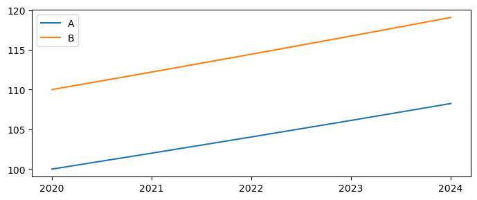
Consider the following concrete example. A DataFrame df has two variables A and B, that each grow by 2% per period, with A initialized at a level of 100 and B at a level of 110 so that we can see each separately on a graph.

df = pd.DataFrame(100.,
     index=[v for v in range(2020,2025)],
       columns=['A','B']) 

df=df.upd("""<2021 -1> A =growth 2
           <2020 -1>   B = 110
          <2021 -1>    B =growth 2
          """)
# Store these variables for later use in comparisons
df['A_ORIG']=df['A']
df['B_ORIG']=df['B']
df

	A	B	A_ORIG	B_ORIG
2020	100.000000	110.000000	100.000000	110.000000
2021	102.000000	112.200000	102.000000	112.200000
2022	104.040000	114.444000	104.040000	114.444000
2023	106.120800	116.732880	106.120800	116.732880
2024	108.243216	119.067538	108.243216	119.067538

    df[['A','B']].plot(xticks=df.index,figsize=(7,3)); #the xticks option forces mathplitlib to only print x-axis values that exist in the index (no decimals)

../../_images/0ae043d40648112ced0d7c11337e36ccc1e029bbfe26d0d8e60b9769fa400f1e.png

The .upd() command below modifies both A and B by adding 5 to their levels in each of 2022 and 2023.

For A, this is done with the keep_growth option set to True – the --kg option in the code below. This means that for A the growth rate after the shock period 2022-23 will be unchanged at 2 percent.

For series B the same shock is applied but with keep_growth set to False using the –nkg option.

The keep_growth global variable is ignored in this instance as each line in the update is overriding it using the –kg option (keep_growth=True) and –nkg option (keep_growth=False).

df=df.upd("""
            <2022 2023> A + 5 --kg
            <2022 2023> B + 5 --nkg
            """)

df[['A','B','A_ORIG','B_ORIG']].plot(xticks=df.index,figsize=(7,3));   

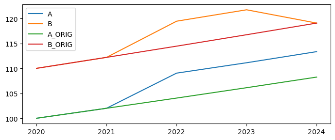
../../_images/393b22a1671a19ea420589aa60daa270a416696fd2fd39cb0946a43bc766e1b0.png

In the first example ‘A’ (the green and blue lines) the level of A is increased by 5 for two periods (2021-2022). The levels of the subsequent values are also increased because the previous growth rate (2%) is now applied to the new higher level of the data in 2022.

For the ‘B’ variable the same level change was input but because of the --nkg (equivalent to keep_growth=False) the periods after the change were unaffected. the shocked variable returns to its pre-shock level immediately in 2023.

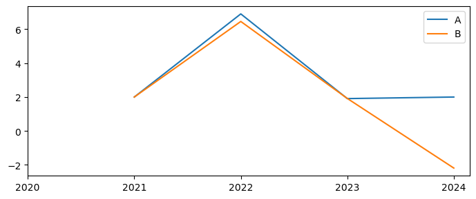
Below are plots the growth rates of the two transformed series.

Here the growth in both series accelerates in 2022, by slightly less than 5 percentage points because a) the base of each is more than 100 in 2021 (because of the 2 percent growth in 2021). Substantially more in the case of B, which was initialized at 110. In 2023 the growth rate of A returns to 2 percent, while the growth rate of B is actually negative because the level (see earlier graph) has fallen back to its original level.

dfg=df[['A','B']].pct_change()*100
dfg.plot(xticks=dfg.index,figsize=(7,3));

../../_images/279fbfe50866871179afcf04c73d03bbe8d7eee215f04bfb693744cb0ec56914.png

1.4.5.2.1. Keep_growth additional examples#

Initialize a new dataframe, with some growth rate

# instantiate a new dataframe with one column 'A' with a value 100 everywhere and index 2020-2025
dftest = pd.DataFrame(100.0,
       index=[v for v in range(2020,2026)], # create row index
       # equivalent to index=[2020,2021,2022,2023,2024,2025] 
       columns=['A'])                                 # create column name
dftest

	A
2020	100.0
2021	100.0
2022	100.0
2023	100.0
2024	100.0
2025	100.0

# Update a to have growth rate accelerationg linearly by 1 from 1 Percent to 5 percent
original = dftest.upd('<2021 2025> a =growth 1 2 3 4 5')  
print(f'Levels:\n{original}\n\nGrowth:\n{original.pct_change()*100}\n')

Levels:
               A
100.000000
101.000000
103.020000
106.110600
110.355024
115.872775

Growth:
        A
NaN
1.0
2.0
3.0
4.0
5.0

Now update A in 2021 to 2023 to a new value

Below performs the same operation twice, the first time the updated value is assigned to the dataframe nkg and the default behavior of keep_growth is False

In the second example the -kg line option is specified, telling ModelFlow to maintain the growth rates of the dependent variable in the periods after the update is executed.

nokg = original.upd('''
<2021 2025>  a =growth 1 2 3 4 5 
<2021 2023>  a = 120  
''',lprint=0)

kg = original.upd('''
<2021 2025>  a =growth 1 2 3 4 5 
<2021 2023>  a = 120  --kg
''',lprint=0)


kg=kg.rename(columns={"A":"KG"})       #rename cols to facilitate display
nokg=nokg.rename(columns={"A":"NOKG"}) #rename cols to facilitate display
df=original.rename(columns={"A":"Orig"}) #rename cols to facilitate display

combo=pd.concat([kg,nokg,df], axis=1)
combo


print(f'Levels\n{combo}\n\nGrowth\n{combo.pct_change()*100}')

Levels
          KG        NOKG        Orig
100.00  100.000000  100.000000
120.00  120.000000  101.000000
120.00  120.000000  103.020000
120.00  120.000000  106.110600
124.80  110.355024  110.355024
131.04  115.872775  115.872775

Growth
        KG      NOKG  Orig
 NaN       NaN   NaN
20.0  20.00000   1.0
 0.0   0.00000   2.0
 0.0   0.00000   3.0
 4.0  -8.03748   4.0
 5.0   5.00000   5.0

Understanding the results

In the first example where KG (keep_growth) was set, the level was set constant for three periods at 120 the rate of growth was 0 for the final two years of the set period. But following this update, the level of A in 2023 is 120. With keep_Growth=True the KG variable growth at 2 percent per year in 2024 and 2025.

In the –nkg example, the levels of NOKG are the same as KG for 2020 through 2023, but because --nkg was selected the levels revert to their pre-shock values, which are lower than the 120 in 2023. As a result the growth rate for NOKG is negative in 2024. The growth rate for 2024 remains 5 because neither the 2024 or 2025 data changed and therefore the 2025 the growth rate does not change.

1.4.5.2.2. keep_growth option set globally#

Above the line level option --keep_growth or --kg was used to keep the growth rate (or not) for a given operation.

This works because by default the global Keep_growth options was set to false. In that context, implementing --kg at the line level temporarily set the keep_growth flag to true for the specific line (and those following).

In the example below we set the keep_growth flag to True globally and then use nkg at the line level.

To set keep_growth to True globally enter it as a specific option for the update command ,keep_growth=True.

In this context, all lines will keep the growth rate (unless overridden at the line level with --nkg or --no_keep_growth).

c,d are updated in 2022 and 2023 and keep the growth rates afterwards
e the --no_keep_growth in this line prevents the updating 2024-2025

# Create a data frame
dftest = pd.DataFrame(100.0,
       index=[v for v in range(2020,2025)], # create row index
       # equivalent to index=[2020,2021,2022,2023,2024] 
       columns=['A','B','C','D','E'])                                 # create column name 
dftest

	A	B	C	D	E
2020	100.0	100.0	100.0	100.0	100.0
2021	100.0	100.0	100.0	100.0	100.0
2022	100.0	100.0	100.0	100.0	100.0
2023	100.0	100.0	100.0	100.0	100.0
2024	100.0	100.0	100.0	100.0	100.0

Note

In the below .upd() command

dfres = dftest.upd('''
<2022 2023> c = 200 
<2022 2023> d = 300  
<2022 2023> e = 400  --no_keep_growth 
''',keep_growth=True)  # <=  Set keep_growth to True for the entirety of the command, 
                       # except for e where it is overridden by the --no_keep_growth flag

There are two keep_growth commands. The final one is the global option (global to the execution of this update). It is passed as an argument to the .upd() method “,keep_growth=True” and applies to every line in the command string (unless overridden). In contrast, the single line command –no_keep_growth is inside the string passed to .upd() and applies only to the line on which it occurs.

dfres = dftest.upd('''
<2022 2023> c = 200 
<2022 2023> d = 300  
<2022 2023> e = 400  --no_keep_growth 
''',keep_growth=True)  # <=  Set keep_growth to True for the entirety of the command, 
                       # except for e where it is overridden by the --no_keep_growth flag
print(f'Dataframe:\n{dfres}\n\nGrowth:\n{dfres.pct_change()*100}\n')

Dataframe:
          A      B      C      D      E
100.0  100.0  100.0  100.0  100.0
100.0  100.0  100.0  100.0  100.0
100.0  100.0  200.0  300.0  400.0
100.0  100.0  200.0  300.0  400.0
100.0  100.0  200.0  300.0  100.0

Growth:
        A    B      C      D      E
NaN  NaN    NaN    NaN    NaN
0.0  0.0    0.0    0.0    0.0
0.0  0.0  100.0  200.0  300.0
0.0  0.0    0.0    0.0    0.0
0.0  0.0    0.0    0.0  -75.0

1.4.5.3. Scale option of the `.upd()` method#

When running scenarios it can be useful to perform sensitivity analyses of model results, to better understand how the model responds when varying the intensity of a shock.

The scale option provides a mechanism for calculating a range of shocks as different proportions of the initially indicated one.

When using the scale option, scale=0 implies no change (effectively the baseline) while scale=0.5 is a scenario half of the full severity.

In the example below .upd() is executed three times for severity equals 0. 0.5 and 1. If the list passed to scale (named severity in this case) had five items in it, the update would be run five times – one time for each item in the list.

This example just prints outputs, a more interesting example would involve the solving a model using these different levels in a series of simulations.

dfinput=df.upd('A = 100')
print(f'input dataframe: \n{dfinput}\n\n')
for severity in [0,0.5,1]: 
    # First make a dataframe with some growth rate 
    res = dfinput.upd('''
    <2021 2025>
    a =growth 1 2 3 4 5 
    b + 10
    ''',scale=severity)
    print(f'{severity=}\nDataframe:\n{res}\n\nGrowth:\n{res.pct_change()*100}\n\n')
    #  
    # Here the updated dataframe is only printed. 
    # A more realistic use case is to simulate a model like this: 
    # dummy_ = mpak(res,keep='Severity {serverity}')    # more realistic 

input dataframe: 
            Orig      A
100.000000  100.0
101.000000  100.0
103.020000  100.0
106.110600  100.0
110.355024  100.0
115.872775  100.0


severity=0
Dataframe:
            Orig      A    B
100.000000  100.0  0.0
101.000000  100.0  0.0
103.020000  100.0  0.0
106.110600  100.0  0.0
110.355024  100.0  0.0
115.872775  100.0  0.0

Growth:
      Orig    A   B
 NaN  NaN NaN
 1.0  0.0 NaN
 2.0  0.0 NaN
 3.0  0.0 NaN
 4.0  0.0 NaN
 5.0  0.0 NaN


severity=0.5
Dataframe:
            Orig           A    B
100.000000  100.000000  0.0
101.000000  100.500000  5.0
103.020000  101.505000  5.0
106.110600  103.027575  5.0
110.355024  105.088126  5.0
115.872775  107.715330  5.0

Growth:
      Orig    A    B
 NaN  NaN  NaN
 1.0  0.5  inf
 2.0  1.0  0.0
 3.0  1.5  0.0
 4.0  2.0  0.0
 5.0  2.5  0.0


severity=1
Dataframe:
            Orig           A     B
100.000000  100.000000   0.0
101.000000  101.000000  10.0
103.020000  103.020000  10.0
106.110600  106.110600  10.0
110.355024  110.355024  10.0
115.872775  115.872775  10.0

Growth:
      Orig    A    B
 NaN  NaN  NaN
 1.0  1.0  inf
 2.0  2.0  0.0
 3.0  3.0  0.0
 4.0  4.0  0.0
 5.0  5.0  0.0

1.4.5.4. lprint option of the `.upd()` method prints pre- and post- update values update#

The lPrint option of the method upd() is set to = False by default. By setting it true, an update command will output the results of the calculation comparing the values of the dataframe (over the impacted period) before, after and the difference between the two.

dfinput.upd('''
# Same number of values as years
<2021 2022> A *  42 44
''',lprint=1);

Update * [42.0, 44.0] 2021 2022
A                    Before                After                 Diff
2021               100.0000            4200.0000            4100.0000
2022               100.0000            4400.0000            4300.0000

1.4.6. The Create option of the `.upd()` determines behavior when a LHS variable does not exist#

By default Create=True. As a result, in the examples above, when a left-hand side variable did not exist the .upd() commands created the previously undeclared variables.

To catch misspellings the parameter create can be set to False. When create=False, if update is executed on a variable that does not exist the specified variable(s) will not be created. Instead, an exception (an error) will be raised alerting to the user that the variable does not exist.

In the example below, the error is captured in a try catch statement (a python method for handling errors) so that the notebook will continue to run despite the error. If the try Catch had not been in place the notebook would stop executing and thrown the error.

Below the cell for reference is the error that would be thrown if the error had not been caught.

try:
    xx = df.upd('''
    # Same number of values as years
    <2021 2022> Aa *  42 44
    ''',create=False)
    print(xx)
except Exception as inst:
    xx = None
    print(inst) 

Variable to update not found:AA, timespan = [2021 2022] 
Set create=True if you want the variable created: 

1.4.6.1. Below the python error generated in the absence of the try / catch expression above.#

Note that the most informative part of the message appears at the end, which is typical of most python errors. The preceding lines give a detailed listing of what steps were being executed when the error was generated which may or may not be of interest.

---------------------------------------------------------------------------
Exception                                 Traceback (most recent call last)
Cell In[15], line 1
----> 1 xx = df.upd('''
      2    # Same number of values as years
      3    <2021 2022> Aa *  42 44
      4    ''',create=False)

File C:\WBG\Anaconda3\envs\ModelFlow\lib\site-packages\ModelFlow-1.0.8-py3.10.egg\modelclass.py:8342, in upd.__call__(self, updates, lprint, scale, create, keep_growth)
   8339 def __call__(self,updates, lprint=False,scale = 1.0,create=True,keep_growth=False,):
   8341     indf = self._obj
-> 8342     result =   model.update(indf, updates=updates, lprint=lprint,scale = scale,create=create,keep_growth=keep_growth,)   
   8343     return result

File C:\WBG\Anaconda3\envs\ModelFlow\lib\site-packages\ModelFlow-1.0.8-py3.10.egg\modelclass.py:1741, in Model_help_Mixin.update(indf, updates, lprint, scale, create, keep_growth)
   1738          multiplier = list(accumulate([(1+i) for i in growth_rate],operator.mul))
   1740 # print(varname,op,value,arg,sep='|')
-> 1741  update_var(df, varname.upper(), op, value,time1,time2 , 
   1742             create=create, lprint=lprint,scale = scale)
   1744  if update_growth:
   1745      lastvalue = df.loc[time2,varname]

File C:\WBG\Anaconda3\envs\ModelFlow\lib\site-packages\ModelFlow-1.0.8-py3.10.egg\modelhelp.py:40, in update_var(databank, xvar, operator, inputval, start, end, create, lprint, scale)
     38 if not create:
     39     errmsg = f'Variable to update not found:{var}, timespan = [{start} {end}] \nSet create=True if you want the variable created: '
---> 40     raise Exception(errmsg)
     41 else:
     42     if 0:

Exception: Variable to update not found:AA, timespan = [2021 2022] 

Recall we have not overwritten df, so the df dataframe is unchanged.

df

	Orig
2020	100.000000
2021	101.000000
2022	103.020000
2023	106.110600
2024	110.355024
2025	115.872775

The .upd() method returns a DataFrame with updated variables.

Contents

1.4. The .upd() method returns a DataFrame with updated variables.#

1.4.1. some examples of the .upd() method#

1.4.1.1. Use .upd to create a new variable#

1.4.2. Multiple updates and specific time periods#

1.4.3. Update several variables in one line#

1.4.4. Operators of the .upd() method#

1.4.4.1. The “=” operator: assign a value(s) to a variable#

1.4.4.2. The “+” operator adds to the existing values in the specified range#

1.4.4.3. The * operator multiplies all values in a range by the specified values#

1.4.4.4. The % operator increases all values in a range by a specified percent amount#

1.4.4.5. The =GROWTH operator sets the percent growth rate to specified values#

1.4.4.6. The +GROWTH operator adds or subtracts from the existing percent growth rate#

1.4.4.7. The =diff operator recursively sets the value of a pre-existing variable to rise or fall by the specified amount#

1.4.5. Options of the .upd() method#

1.4.5.1. The keep_growth option (–kg and –nkg)#

1.4.5.2. The default keep_growth behavior#

1.4.5.2.1. Keep_growth additional examples#

1.4.5.2.2. keep_growth option set globally#

1.4.5.3. Scale option of the .upd() method#

1.4.5.4. lprint option of the .upd() method prints pre- and post- update values update#

1.4.6. The Create option of the .upd() determines behavior when a LHS variable does not exist#

1.4.6.1. Below the python error generated in the absence of the try / catch expression above.#

1.4. The `.upd()` method returns a `DataFrame` with updated variables.#

1.4.1. some examples of the `.upd()` method#

1.4.1.1. Use `.upd` to create a new variable#

1.4.4. Operators of the `.upd()` method#

1.4.5. Options of the `.upd()` method#

1.4.5.3. Scale option of the `.upd()` method#

1.4.5.4. lprint option of the `.upd()` method prints pre- and post- update values update#

1.4.6. The Create option of the `.upd()` determines behavior when a LHS variable does not exist#