The Interface
Learning objective
By the end of this page you'll be able to open GeoE3, create a new analysis project from a boundary layer, choose the right scale for your study area, set up a routing environment, and read the dock's tree view, including the status icons and right-click menu every other page in this walkthrough relies on.
This page assumes you've already installed QGIS and the GeoE3 plugin and have some data to work with. If not, see Getting Data first.
Opening the plugin
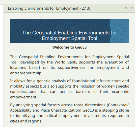
Once installed, you'll find GeoE3's icon in the QGIS toolbar. Click it to open the panel, which docks to the right-hand side of the window by default.
The first page is a short welcome and overview; the next explains what the tool does and who built it. Use the arrow buttons at the bottom of the panel to move between pages.
Opening or creating a project
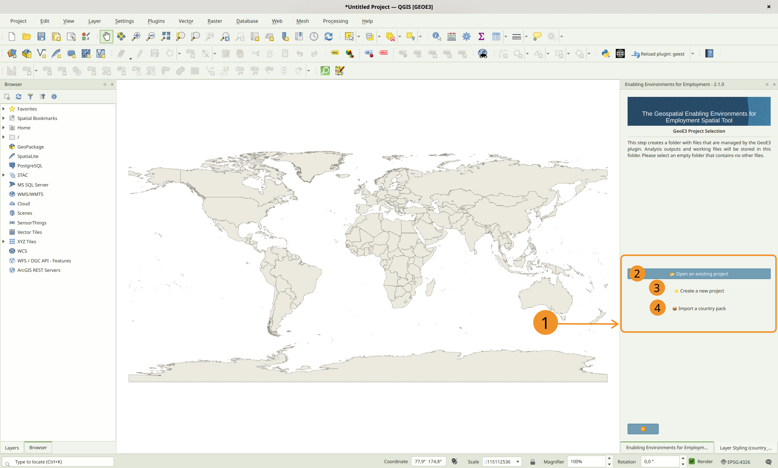
Next, GeoE3 asks you to choose a project folder. Every analysis lives in its own folder, which the plugin manages for you.
Open an Existing Project loads a project folder you've already set up and configured. Pick this to carry on where you left off.
Create a New Project walks you through setting one up from scratch, which is what the rest of this page covers.
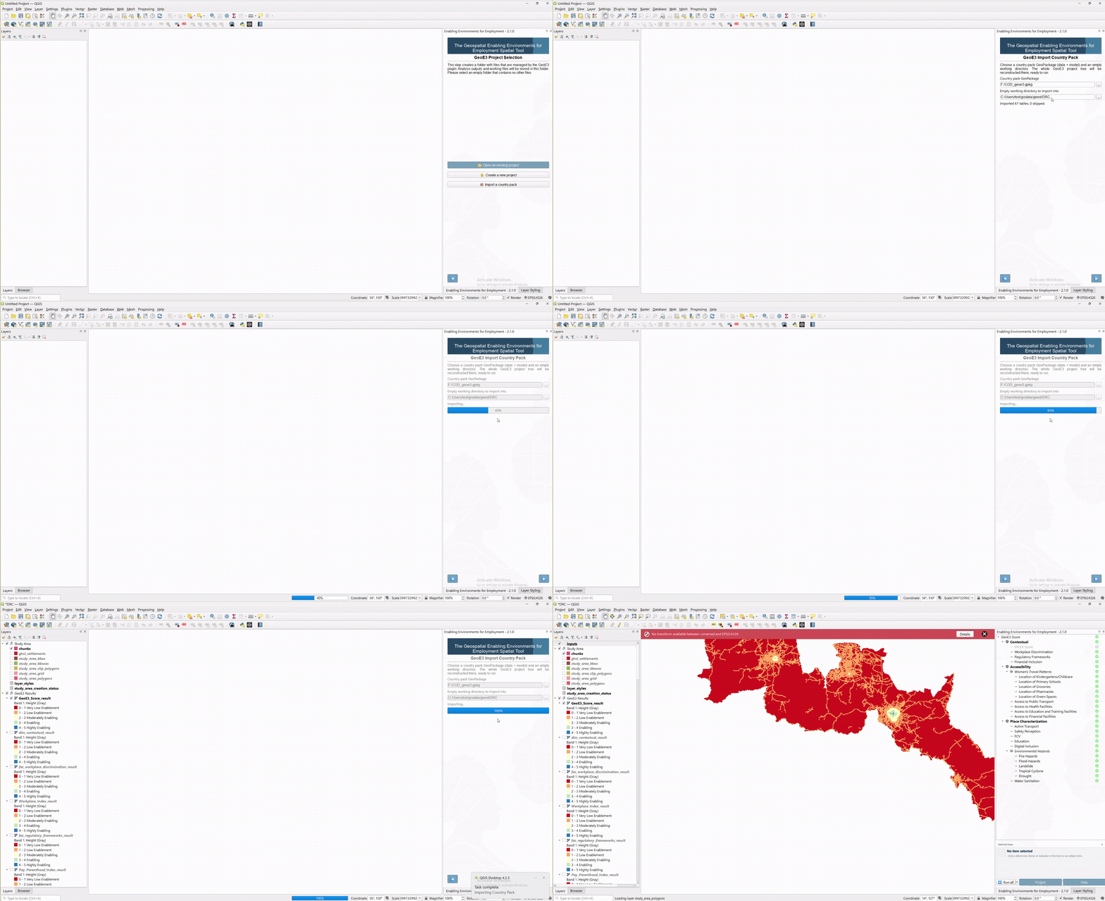
Import a Country Pack rebuilds someone else's project from a single GeoPackage they exported (see Building a Country Pack, later in this walkthrough). Point it at the pack file and an empty working folder. GeoE3 reconstructs the project there including the study area, each input's configuration, all of the already-computed results, and the model itself.
Warning
The folder you choose must be empty. GeoE3 treats everything in it as its own. Using a folder that already has other files in it can lead to errors or accidental overwrites. Give it a descriptive name (country/region plus a date is a good pattern) so you can find it again later.
Creating a new project
Choose Create a New Project, then browse to the empty working folder you made earlier and use that as the project folder. Then you've got three choices to pick from to define the scale of your analysis:
| Scale | Typical use | Default grid size |
|---|---|---|
| Regional | Quick analysis, multi-country or continental study | ~30 km (hex grid) |
| National | A single country | 1,000 m (1 km) |
| Local | A city or small region | 100 m |
In all three cases you can change the grid size if you want to, but the defaults are a reasonable place to start.
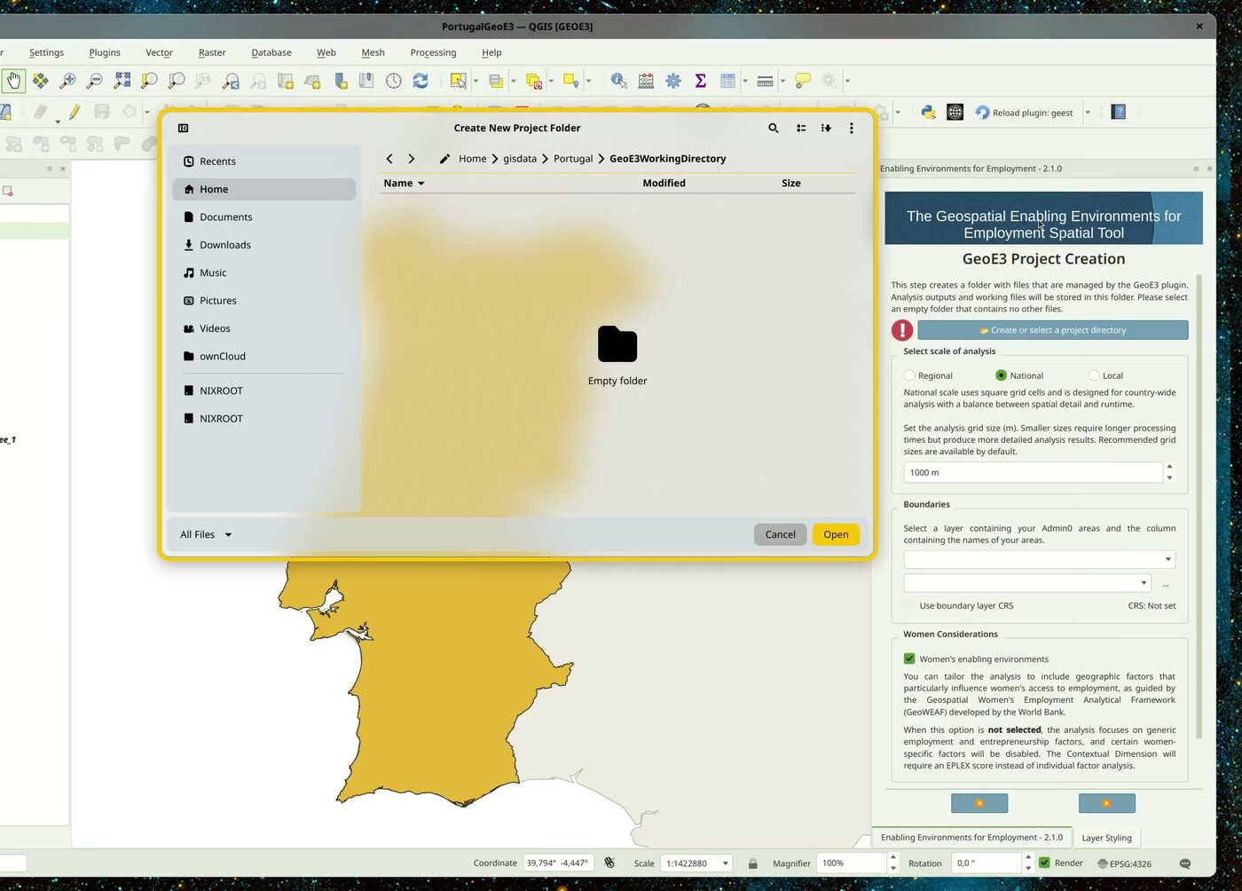
Then it asks for the boundary layer. Point it at your Admin0 (national boundary) layer, and tell it which column has the country name. If your boundary layer doesn't look like the typical boundary you'd expect (it still extends out into the ocean, for example, or is missing the level you need), see the GADM and HDX tutorials. OpenStreetMap's admin boundaries aren't always reliable.
The last thing it asks is whether you want to do a Women's Enabling Environment study, or just a generic economic enabling-environment study. Leave Women's Enabling Environments ticked for the GeoWEAF-framework analysis this walkthrough demonstrates; untick it for the generic one, and you'll get a slightly different workflow. Some women-specific factors get disabled, and the Contextual dimension needs an EPLEX score instead of individual factor analysis.
What happens next: the study area grid
Once you confirm, it computes a grid across the study area and writes that into a GeoPackage file. You can see it in the study area. It creates various different products: the main thing is the GeoPackage, which contains a regular grid (for a regional analysis this is an H3 grid, so hexagons covering the whole study area; national and local scale use square grid cells instead), and it also contains masks. A mask is a raster layer which covers the study area, excluding any pixels outside the area by giving them NoData, and including any areas inside the study area by giving them a value of one.
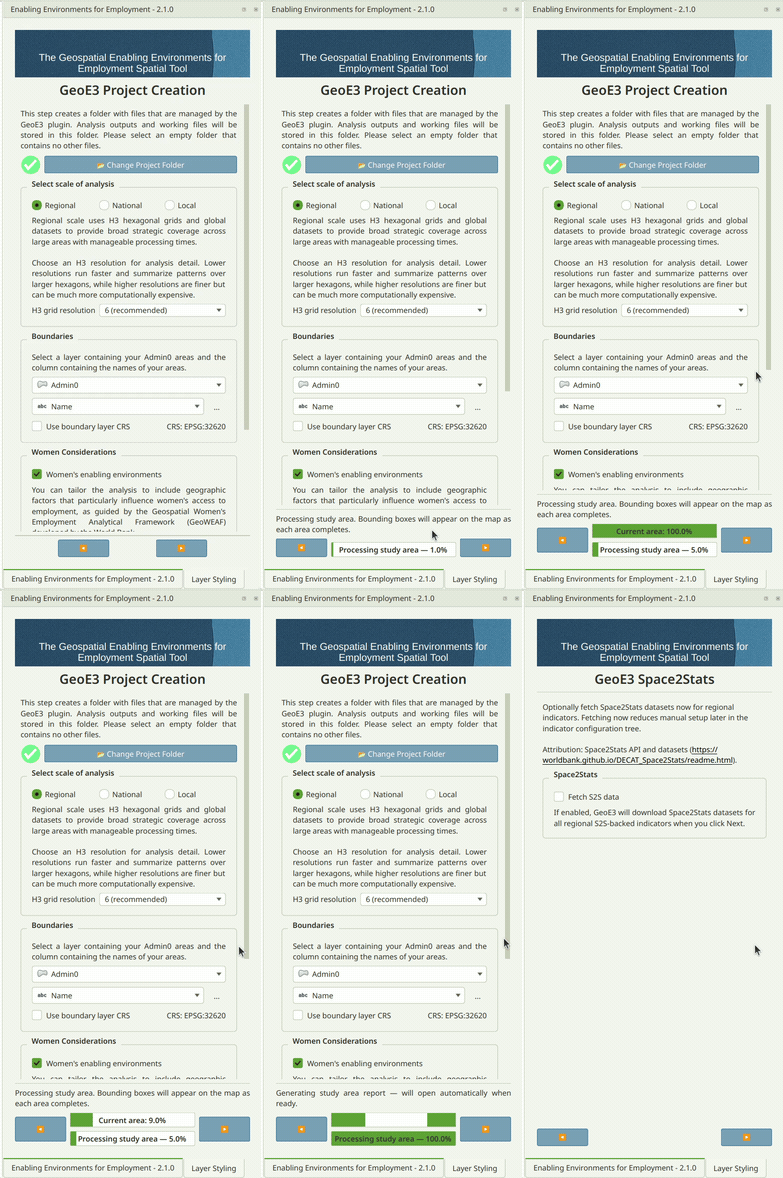
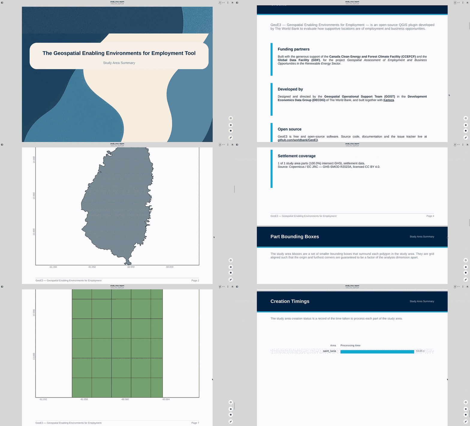
When it finishes, a Study Area Report opens automatically, summarizing
how many grid cells were created, how long each part of the country took
to process, and where the generated files live (your project folder's
study_area/ subfolder). You can reopen it any time.
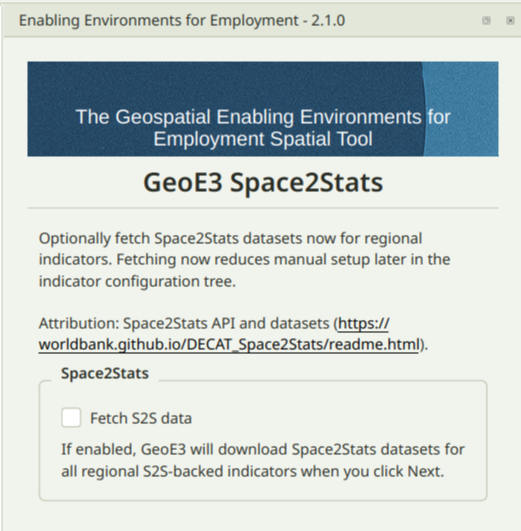
If you picked Regional scale, GeoE3 now offers to prefetch Space2Stats data for every Space2Stats-backed indicator in one go. Tick Fetch S2S data and click Next. National and local-scale projects skip this step entirely. See Getting Data for exactly what gets downloaded.
Setting up routing
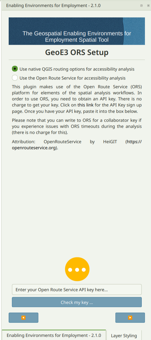
The next thing it wants to do is set up the routing environment. For some
analysis steps we use a routing analysis that allows us to understand,
for example, what's the travel time for a woman to move from her home to
a clinic (or what have you) using the road network. It's possible to use
OpenRouteService for this, but you need an API key. Or you can use the
native QGIS routing (native:serviceareafromlayer), which is a bit
slower but doesn't require any keys.
Next you should indicate if you've got a road network. If you've already downloaded OSM data (see Getting Data), you can use the road lines layer it provides. If you don't have a road dataset, you can also click the Download from OpenStreetMap button and it will fetch a combined roads and cycleways network for you from OpenStreetMap directly.
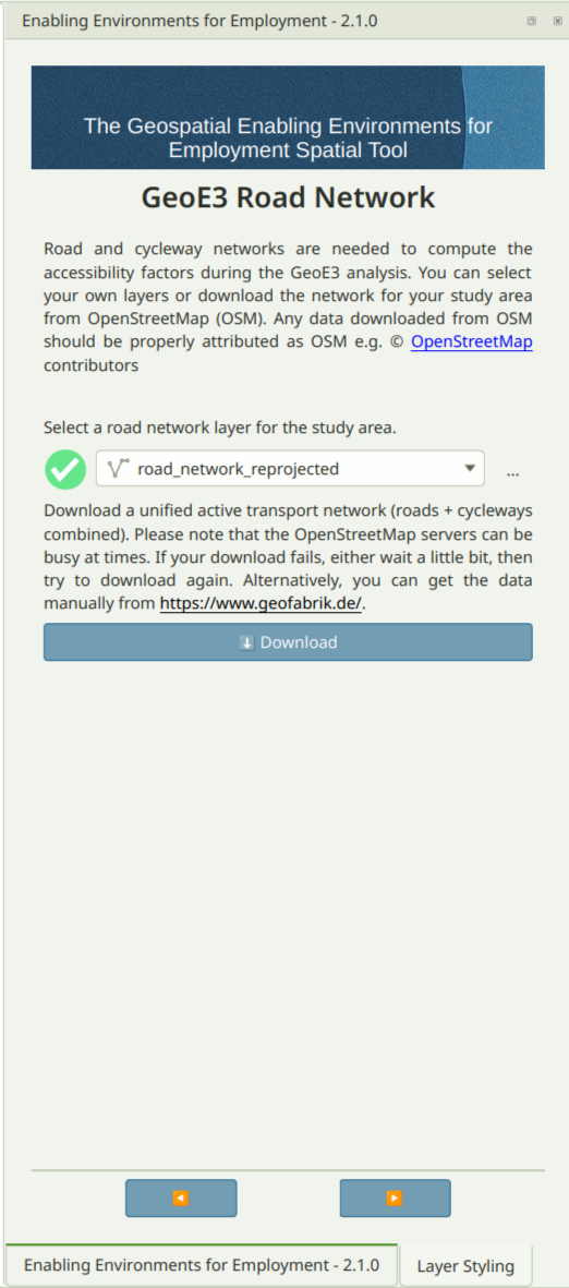
Note
If your road network layer isn't already in the study area's CRS,
GeoE3 reprojects it for you automatically. You'll see the
reprojected copy named with a _reprojected suffix, like
road_network_reprojected above.
Reading the dock: a tree of dimensions, factors and indicators
Once you click through, you land on the model tree (the main working view you'll spend most of your time in). It organises the different types of analysis outputs into three categories, which we call dimensions: the Contextual dimension, the Accessibility dimension, and the Place Characterization dimension. Those are further subdivided into factors (the second-level grouping), and each dimension may have one or more factors associated with it.
It's a tree in the literal QGIS-layer-panel sense: expand a dimension to see its factors, expand a factor to see its indicators. What each of these levels actually means, and how they combine, is the subject of The Model. This page is just about finding your way around the panel itself.
Each row's small leading icon also shows what kind of item it is:
| Icon | Role |
|---|---|
 |
Dimension |
 |
Factor |
 |
Indicator |
Status widgets. Each row in the tree also shows a small status icon telling you what state that item is in:
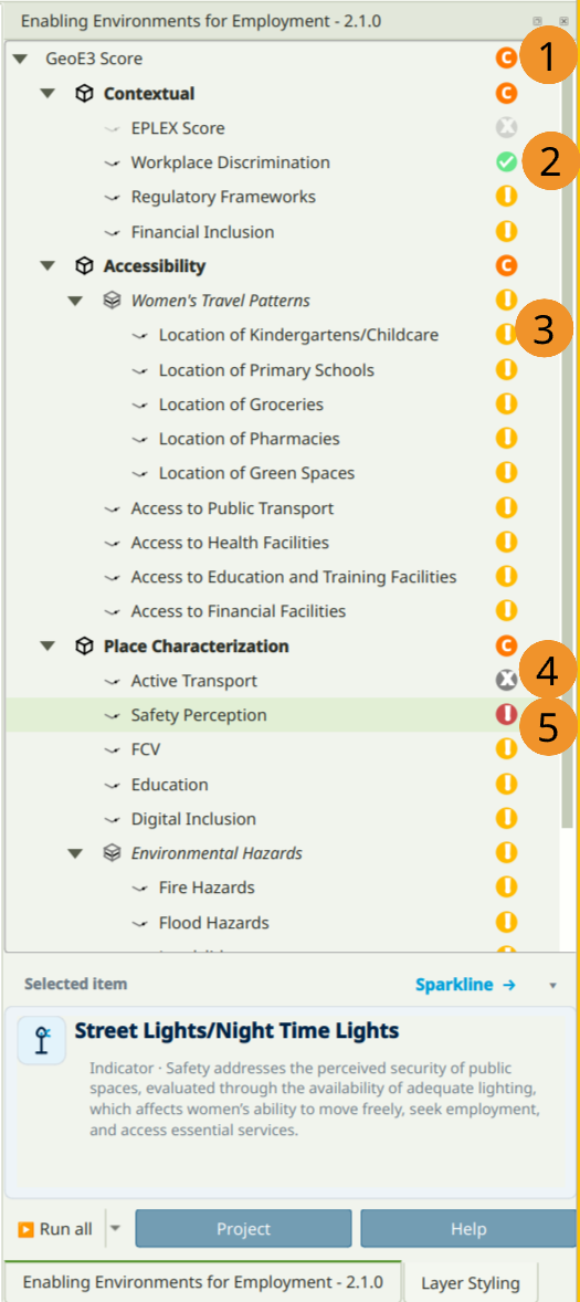
| # | Icon | Status | Meaning |
|---|---|---|---|
| 1 |  |
Configured and ready to run | Inputs are set up. The workflow hasn't run yet. |
| 2 |  |
Completed successfully | Processing finished without errors. |
| 3 |  |
Not yet configured | Required inputs are still missing. |
| 4 |  |
Disabled | Deliberately excluded. Won't run or count toward the score. |
| 5 |  |
Completed with error | Something went wrong. Check the log file. |
Note
In this example, EPLEX Score shows as Disabled because this is a Women's Enabling Environments analysis, which uses the WBL-based indicators instead (see Contextual Dimension). A generic economic-enablement analysis is the other way around: EPLEX Score is enabled, and the WBL indicators are disabled.
Right-click to interact with items
Every item in the tree (indicator, factor, dimension or the top-level analysis) responds to the same right-click context menu. This is how you drive the whole tool once an item is configured:
| Menu item | What it does |
|---|---|
| Run Item Workflow | Executes that item's workflow, computing its output |
| Clear Item | Removes the item's results so you can reconfigure and rerun it |
| Clear Results | Clears all previously generated results |
| Show Attributes | Displays detailed attribute data for the item |
| Add to Map | Adds the item's output layer group to the QGIS Layer Panel |
| Open Log File | Opens the log file to review the workflow's detailed processing or errors |
| Open Working Directory | Opens the folder containing that item's output files |
The successful completion of a workflow is always shown by a green checkmark status widget. If results don't automatically appear in the Layer Panel after processing, right-click the item and choose Add to Map.
Tip
If an input value needs to change for any reason (an incorrect initial entry, say), right-click the item and choose Clear Item, then right-click it again and, while holding Shift, choose Run Item Workflow. This reassesses the input and outputs the corrected score.
The top-level analysis item's right-click menu adds several more entries on top of the common set above:
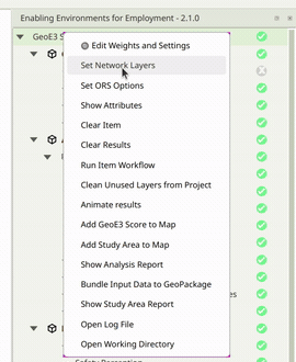
| Menu item | What it does |
|---|---|
| Edit Weights and Settings | Opens the dialog for adjusting the analysis's dimension weights and other settings |
| Set Network Layers | Jumps to the Network tab to configure the road network used for routing |
| Set ORS Options | Jumps to the OpenRouteService tab to set up routing options |
| Clean Unused Layers from Project | Removes any layers left in the QGIS project that are no longer in the legend |
| Animate results | Steps through all tree items in sequence with a short pause on each, as a visual tour of the run |
| Add GeoE3 Score to Map | Loads the GeoE3 Score layer onto the map |
| Add Study Area to Map | Loads the study area boundary and grid layers onto the map |
| Show Analysis Report | Generates and opens the full PDF analysis report |
| Bundle Input Data to GeoPackage | Packages all configured input datasets into a single GeoPackage |
| Show Study Area Report | Generates and opens the study area summary report |
Run All (bottom of the panel) runs every workflow regardless of status; Run Incomplete only runs the ones that haven't completed yet. The Project button takes you back to the setup pages above if you need to change the scale or boundary layer later, and Help opens the plugin's GitHub documentation.
Configuring every item in this tree (pointing each factor at its data, or entering a researched national score) is exactly what The Model, Processor Types and Configuring Items walk through next.
Recap
- GeoE3 projects live in their own empty folder; pick Create a New Project to start one from a boundary layer.
- The scale you choose (regional/national/local) sets a default grid size and, for regional, unlocks the Space2Stats prefetch.
- Routing for accessibility indicators defaults to QGIS's free native engine; OpenRouteService is faster but needs an API key.
- The dock is a tree (dimension → factor → indicator), and every row has a status icon and the same right-click menu: Run Item Workflow, Clear Item, Add to Map and the rest.