Viewing Your Results
 Viewing Your Results
Learning objective
By the end of this page you'll be able to interpret the final GeoE3 score, drill into any dimension, factor or indicator's methodology, weightings and score distribution, step through the GeoE3 Score's output carousel, and understand the bivariate legend that results from combining enablement with population density.
We assume the GeoE3 Score has been configured and run (see Configuring Items for assigning dimension weights, adding a population layer or mask, and Running the Analysis for actually kicking off the run). The outputs identify regions where conditions are optimal, or at least favorable, for women to access job opportunities in a specific sector, highlighting key infrastructure investments that could boost women's participation in the workforce.
Once every dimension has been processed (see the three previous pages) and the GeoE3 Score has run, a new layer appears at the analysis node. It's on the same Likert scale as everything underneath it: red cells are very low economic enablement, orange is low, yellow is intermediate, green is enabling, and blue is very enabling.
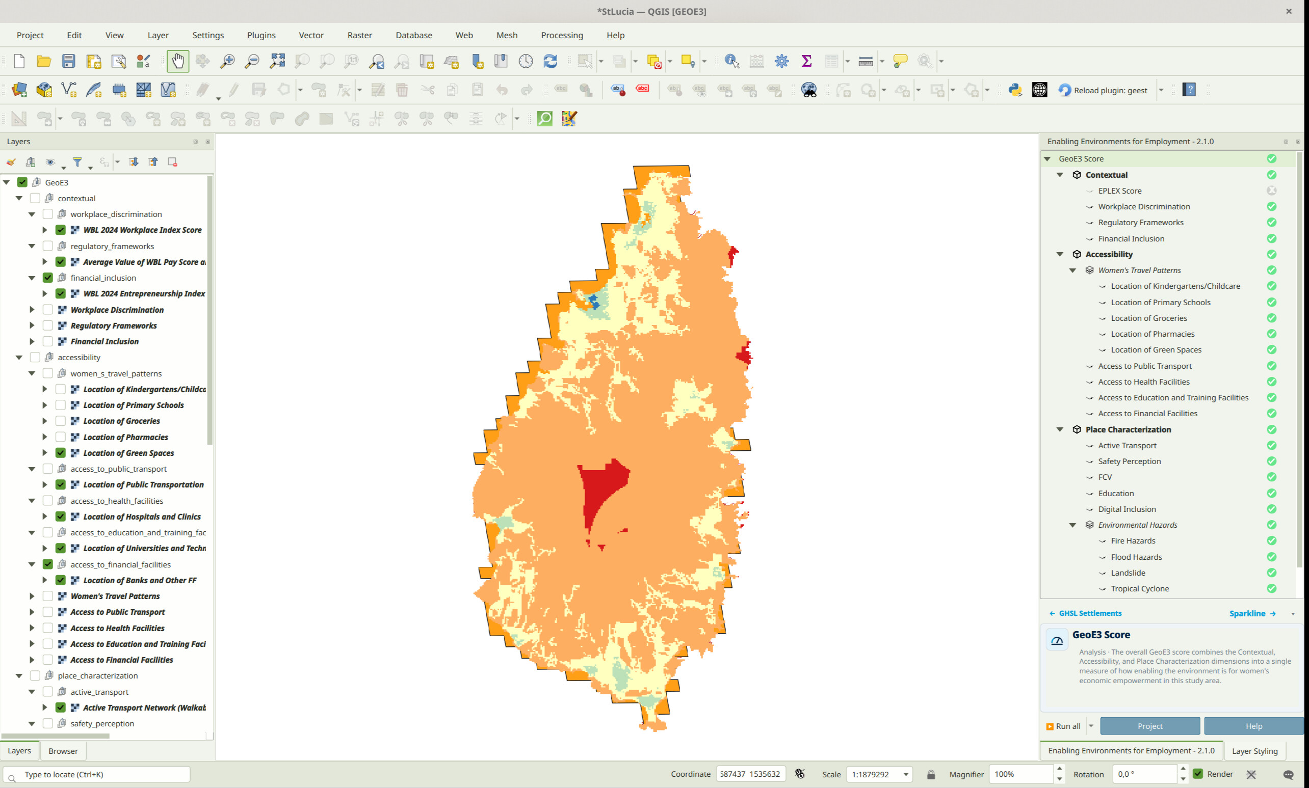
We're able to go and explore all of the individual results as well. Click on any layer in the tree. You'll see a description of it in the info panel at the bottom right. You can shrink this panel using the little triangle icon and resize it back again using the same icon. For every indicator, factor and dimension, that description now comes with extra pages. Step through them using the → link in the panel's header.
You can go through and explore the different results generated at the dimension level, then the factor level, and down to the indicator level. Remember that the combination of indicators is combined into the factor. If you double-click on a factor, you can see a table with the weightings used to show what the relative importance of each was in the total assessment. This is the same weights dialog covered in Configuring Items.
Exploring an Item: Description, Methodology and Score Distribution
Click an indicator, for example, Workplace Discrimination. The info panel opens on its Item page. You'll see its role, its description, and a Methodology → link.
Click Methodology →. The panel explains, in plain language, which of the eight processor types produced this indicator's score. It's the same explanation the PDF report's Methodology section gives.
Click forward once more and you'll reach the Sparkline. It's a small bar chart showing how the grid cells scored, 0 to 5, for whatever you've got selected. Factors and dimensions skip straight here from their Item page since they do not have a methodology page.
The header's left hand label walks you back the same way you came. One click from Sparkline takes you back to Methodology for an indicator, or straight to Item for a factor or dimension. Select a different item while you're on the Methodology page and the panel stays on Methodology for the new item too, as long as it still has one. It behaves like a tab that stays selected as you move around the tree.
The GeoE3 Score's Own Carousel
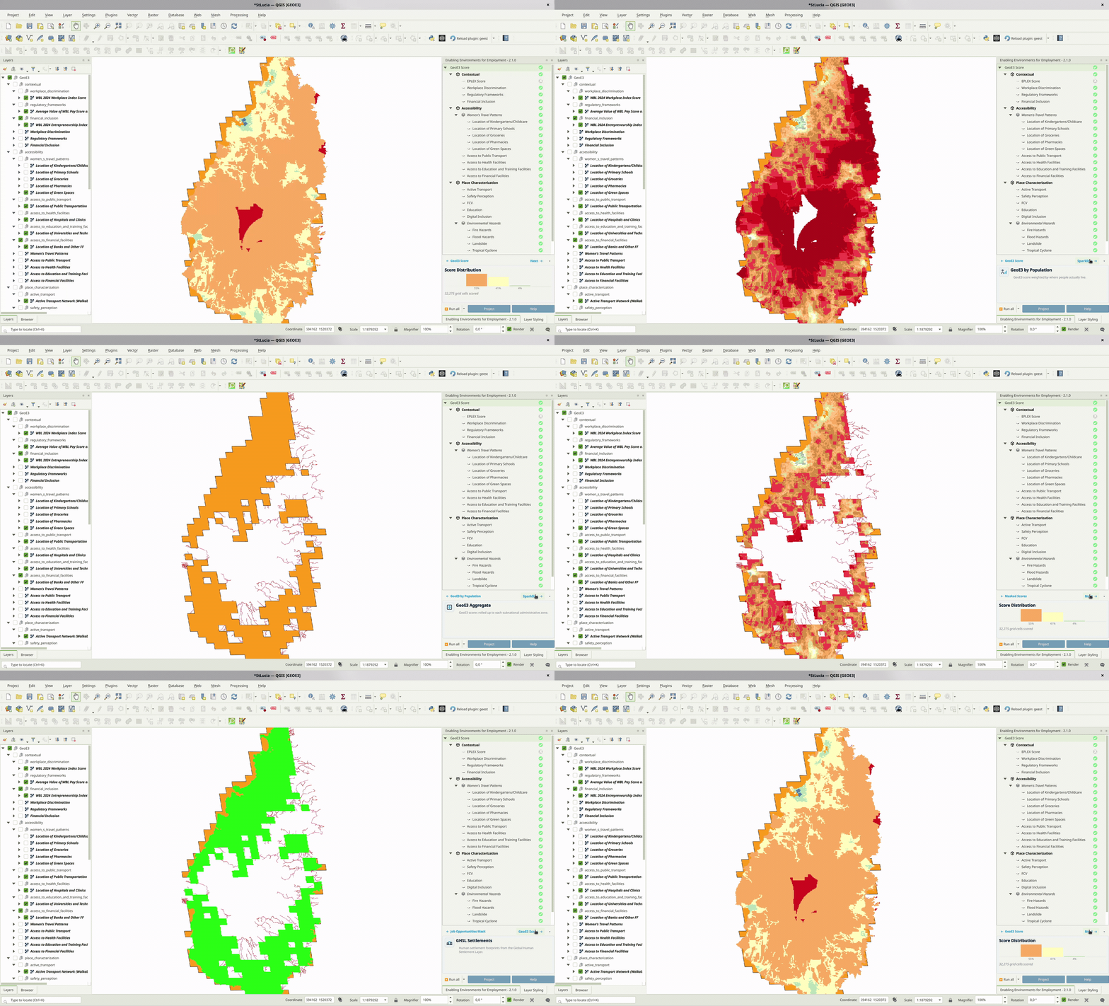
The GeoE3 Score node works a little differently. A single run produces up to six different output layers. Click it and the same → link cycles through all six. GeoE3 Score. GeoE3 by Population. GeoE3 Aggregate. Masked Scores. Job Opportunities Mask. GHSL Settlements. You'll only see the ones you actually configured and ran.
Each stop gets its own Item page. Four of the six also get their own Sparkline. Job Opportunities Mask is a binary mask. GHSL Settlements is a reference layer. Neither gets a Sparkline page. So "Next" from the GeoE3 by Population stop goes to that stop's own score distribution first. Then it moves on to Aggregate.
Visualizing the Outputs
When completing the process, the outputs are automatically added to the Layer Panel in QGIS as a group layer. This group layer has the Mutually Exclusive Group feature activated, which ensures that only one layer within the group can be visible at a time. When this feature is enabled, turning on the visibility of one layer automatically turns off the visibility of the others within the same group, making it easier to compare results without overlapping visualizations.
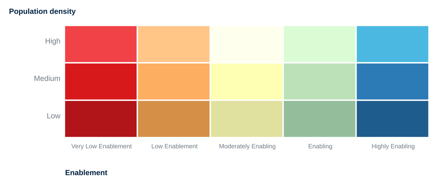
The outputs consist of all GeoE3 score outputs (aggregated at administrative level, by population, or by job distribution). The aggregated-by-population outputs use a bivariate legend: 5 enablement levels × 3 population tiers, 15 exact classes in total:
| Score | Class | Colour |
|---|---|---|
| 1 | Very low enablement, low population | |
| 2 | Very low enablement, medium population | |
| 3 | Very low enablement, high population | |
| 4 | Low enablement, low population | |
| 5 | Low enablement, medium population | |
| 6 | Low enablement, high population | |
| 7 | Moderately enabling, low population | |
| 8 | Moderately enabling, medium population | |
| 9 | Moderately enabling, high population | |
| 10 | Enabling, low population | |
| 11 | Enabling, medium population | |
| 12 | Enabling, high population | |
| 13 | Highly enabling, low population | |
| 14 | Highly enabling, medium population | |
| 15 | Highly enabling, high population |
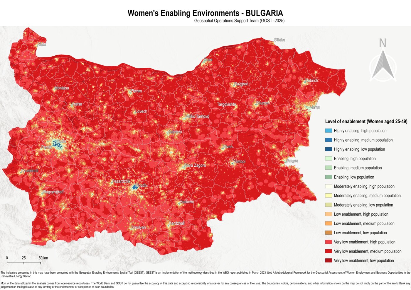
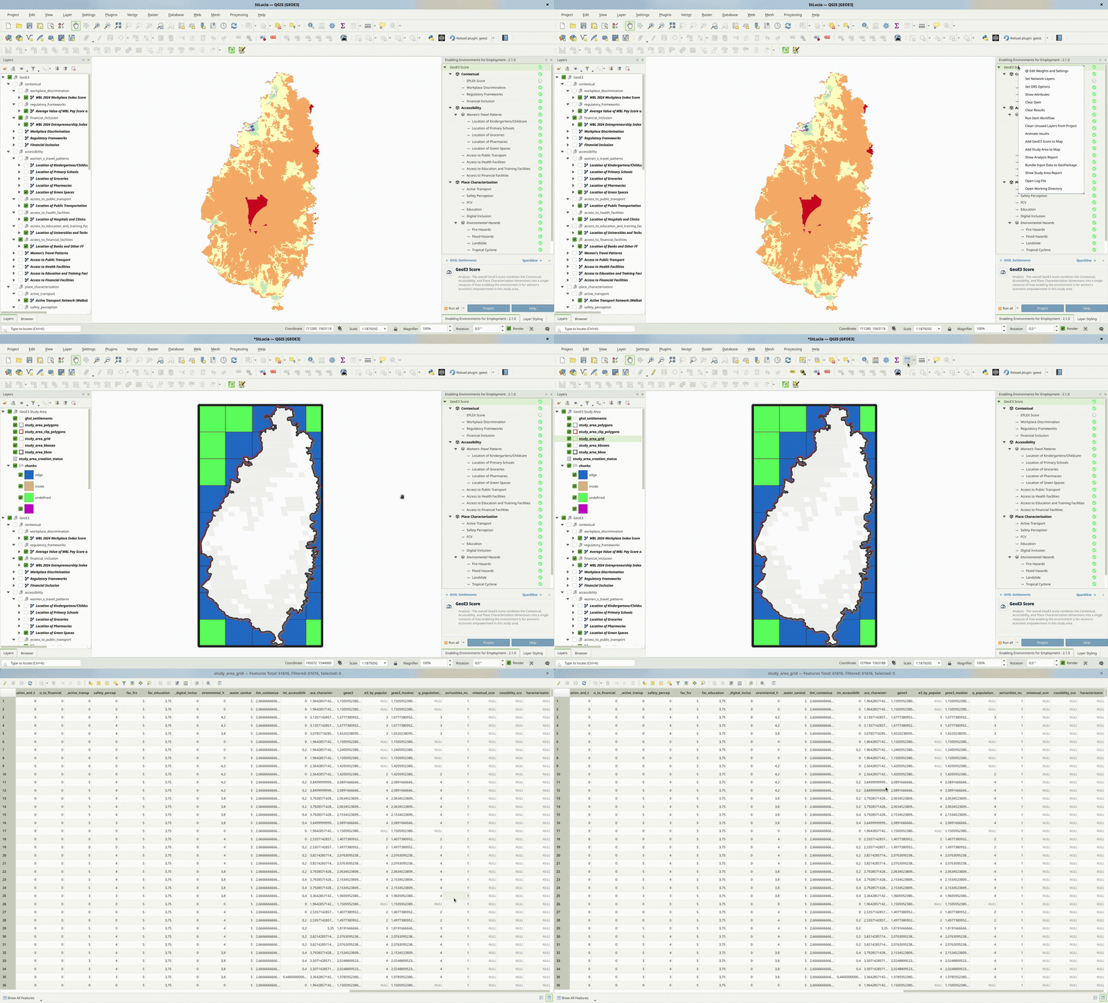
The outputs are stored within the project folder created during the setup phase as raster files and as columns in the study_area_grid table in the study_area.gpkg. The process for adding the study area grid to your QGIS project is shown in the image below.
These files can be shared and further utilized for various purposes, such as visualization in QGIS or other GIS software, integration into reports, overlaying with other spatial datasets, or performing advanced geospatial analyses, such as identifying priority areas or conducting trend analysis based on the scores.
If the results do not immediately appear in the Layer Panel after processing the GeoE3 Scores, you can resolve this by either adding them manually from the folder path or by right-clicking on the GeoE3 Score and selecting Add to map from the context menu.
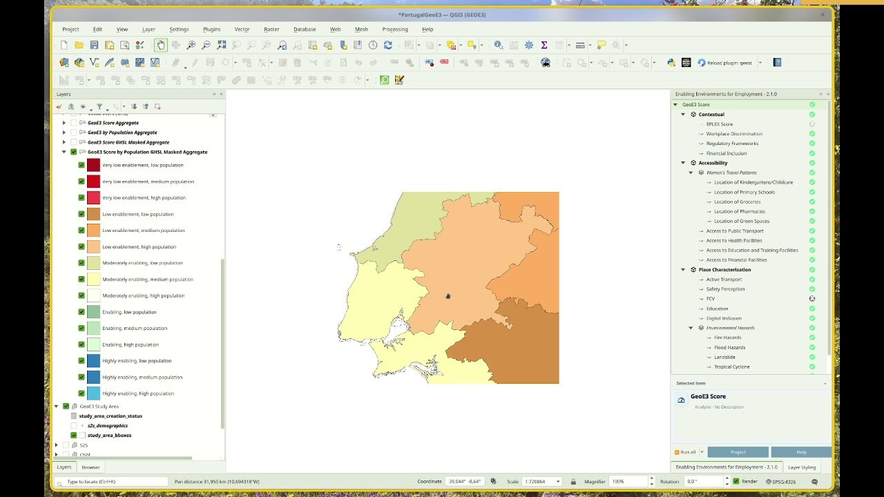
When population and a subnational boundary layer are both configured, Add GeoE3 Aggregates to Map breaks the enablement scores down by subnational districts using the same 15-class bivariate legend above. Each region is shaded by its majority class, from dark red (low enablement, low population) through to bright blue (high enablement, high population).
There's one more advanced option worth knowing about: the subnational score matrix. It's covered in The Analysis Report along with the rest of what's in the PDF report.
The GeoE3 Score node still keeps two dedicated actions on its right-click menu: Add GeoE3 Score to Map and Add Study Area to Map. The other five outputs (By Population, Aggregates, Masked Scores, Job Opportunities Mask, GHSL Settlements) can be viewed using the info panel's carousel, covered above in The GeoE3 Score's Own Carousel. The first time you land on a stop it loads onto the map. After that, revisiting it just switches its visibility back on.
Every run also produces a full PDF analysis report, and the raw grid results are available for export to CSV or any GIS format. Both are covered next, in The Analysis Report.
Recap
- The info panel's → link steps any indicator through Item, Methodology and Sparkline. Factors and dimensions skip straight from Item to Sparkline.
- The GeoE3 Score node has its own carousel of up to six output stops, each with its own Item page and, for four of the six, its own Sparkline.
- The GeoE3 Score combines the three dimensions you've already configured, weighted and run just like any other item in the tree.
- Adding a population layer (auto-fetched from Space2Stats, or your own, see WorldPop) unlocks the 15-class bivariate legend: 5 enablement levels × 3 population tiers.
- Adding a subnational boundary layer breaks results down by region; adding a mask (GHSL settlements, or your own) restricts the analysis to areas you actually care about.
- The Subnational score matrix setting (Settings → Options → GeoE3, off by default) adds a region-by-factor breakdown table to the PDF report.