Methodological Framework#
The objective of this analysis is to construct an Urban Space Usage Index that captures how different parts of a city are used over time.
Specifically, the analysis aims to: (i) quantify the intensity of visits to each spatial unit; (ii) detect deviations from typical mobility patterns; (iii) interpret such deviations in response to both planned events and unpredictable events.
The analytical framework is based on the following principle:
This approach is consistent with state-of-the-art methodologies in mobility analysis and crisis monitoring, where deviations from typical mobility conditions are used as proxies for behavioral change and system disruption [DWE15, YJLG+21].
1. Data Source#
The analysis is based on the Veraset Movement dataset, provided by Veraset as part of the Mobility Data collection from the Development Data Partnership. This dataset consists of anonymized, high-frequency mobile device location pings collected through a network of mobile applications and software development kits (SDKs). Each record includes geographic coordinates (latitude and longitude), a UTC timestamp, and a device identifier.
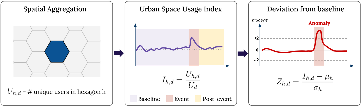
Observations are spatially aggregated using the Uber H3 hierarchical spatial index. For each hexagon \(h\) and day \(d\), we compute the number of unique users visiting the hexagon. Data are aggregated at a daily temporal resolution.
2. Methodology#
The goal of the analysis is to detect deviations in spatial activity relative to typical conditions.
To study an event, we define the following temporal windows:
Baseline period: represents typical, stable, and event-free conditions;
Event period: the time during which the event occurs, when deviations are expected;
Post-event period: used to assess recovery dynamics, especially in applications concerned with economic recovery and resilience.
The baseline defines expected activity levels and variability, while the event and post-event periods are used to quantify deviations and assess their magnitude and duration.
2.1 The Urban Space Usage Index#
To quantify the activity level of each spatial unit (H3 hexagon), we define daily activity as the number of unique users visiting that location:
where \(U_{h,d}\) is the number of unique users in hexagon \(h\) on day \(d\). This metric captures the intensity of human presence.
However, as a raw count, \(A_{h,d}\) is sensitive to fluctuations in the total number of active users. As a result, temporal variations in \(A_{h,d}\) may reflect changes in data coverage rather than true mobility dynamics, potentially leading to misleading interpretations.
To account for this variability, we define the Urban Space Usage Index (I) as the normalized activity level of each spatial unit:
where \(U_d\) is the total number of active users on day \(d\).
This index represents the share of total observed activity occurring in hexagon \(h\) on day \(d\), capturing relative spatial usage independently of fluctuations in data volume.
This normalization controls for day-to-day variability and enables consistent comparisons over time. In the remainder of the analysis, \(I_{h,d}\) is used as the primary measure of urban space usage.
2.2 Baseline Estimation#
For each hexagon \(h\), we compute the following statistics over the baseline period:
Mean activity: \(\mu_h\), defined as the average of \(I_{h,d}\) during the baseline period.
Standard deviation: \(\sigma_h\), defined as the standard deviation of \(I_{h,d}\) during the baseline period.
These quantities represent the expected level and variability of mobility activity under typical conditions for each spatial unit \(h\), and serve as the reference against which deviations are evaluated.
2.3 Deviation Measurement (Z-score)#
While the Urban Space Usage Index captures the level of spatial activity, deviations from typical conditions are assessed through its standardized form (z-score), enabling the detection of anomalous patterns.
To assess whether mobility activity during the event period deviates from baseline conditions, we compute a z-score for each hexagon \(h\) and day \(d\) in the event (or post-event) period as follows:
The z-score measures how many standard deviations the observed activity deviates from its expected baseline.
Interpretation:
\(Z \approx 0\): typical activity
\(Z > 0\): above-average activity
\(Z < 0\): below-average activity
Thresholds for anomaly detection:
\(|Z| > 1\): moderate deviation
\(|Z| > 2\): strong deviation
\(|Z| > 3\): extreme anomaly
Negative values may indicate reduced activity or accessibility, while positive values may reflect increased concentration or displacement of activity. When a post-event period is available, recovery dynamics can be assessed by tracking how quickly \(Z_{h,d}\) returns toward zero and by measuring the duration of anomalous conditions.
3. Limitations and Assumptions#
Despite its robustness and widespread adoption, the methodology is subject to several limitations:
Sampling bias: mobility data represents only a subset of the population and may not be fully representative.
Temporal variability in user base: normalization mitigates this issue but may not fully eliminate residual effects.
Multi-location visits: users may visit multiple hexagons within a day; the index reflects spatial coverage rather than exclusive presence.
Baseline sensitivity: results depend on the choice of baseline period; atypical baseline conditions may affect interpretation.
External confounders: observed deviations may be influenced by factors unrelated to the event of interest (e.g., holidays, policy changes).
Despite these limitations, the framework provides a consistent, scalable, and interpretable approach for monitoring changes in urban mobility and space usage.