Urban Activity Dynamics During 2023 Heatwaves in Manila

In this case study, we apply our methodology to anonymized mobility data from Veraset to assess the impact of a climate shock, specifically an extreme heatwave, on urban activity patterns. Understanding how populations move and use urban spaces during extreme heat provides insights into behavioral adaptation, infrastructure resilience, and urban climate vulnerability. We focus on a series of heatwave days in late April 2023 (i.e., April 20, 21, 23, 28, and 30) that affected Manila (Philippines). Using the Urban Space Usage Index, we quantify deviations from typical activity patterns and examine how urban areas respond to this climate shock.

1. Data

1.1 Mobility Dataset

The analysis is based on the Veraset Movement dataset, provided by Veraset as part of the Mobility Data collection from the Development Data Partnership. The dataset consists of anonymized mobile device location pings collected via a network of mobile applications and software development kits (SDKs). Each record includes geographic coordinates, a timestamp, and an anonymized device identifier. These data provide large-scale observations of human mobility, enabling the analysis of spatial and temporal patterns of urban activity.

1.2 Area of Interest (AOI)

The analysis focuses on the metropolitan area of Manila (Metro Manila), the capital region of the Philippines. The study area is defined using administrative boundaries extracted from OpenStreetMap (OSM) (Figure 1).

Figure 1. Administrative boundary of the metropolitan area of Manila (Metro Manila), used to define the area of interest (AOI). All mobility data are spatially clipped to this region and aggregated using the H3 hierarchical grid system.

We spatially discretized the area of interest using the H3 Uber hierarchical indexing at resolution 8, corresponding to hexagonal cells of approximately 0.737 km². Each H3 cell (or hexagon) represents the spatial unit of the analysis.

1.3 Time window and study periods

To capture mobility and activity dynamics associated with extreme heat, we extract data for the period April 3-30, 2023, spatially clipped to the study area.

We define two analysis periods:

• Baseline period: April 3-11*

• Event period: heatwave days, namely April 20, 21, 23, 28, and 30.

The extracted dataset consists of approximately 102 million GPS points generated by 994,400 unique users.

* We exclude the period 12-19 April from the baseline, as it is associated with anomalously high activity levels (see Figure 4), likely driven by exogenous events. Including these days would bias the baseline and inflate Z-score magnitudes; therefore, they are omitted to ensure a more stable and representative reference period.

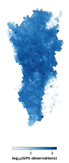
Figure 2. Spatial distribution of GPS observations shown as the average number of records per H3 hexagon (resolution 8). Higher values represent a greater concentration of recorded activity. The color scale is log₁₀-transformed, with darker blue tones indicating areas with more observations.

1.4 Preprocessing and filtering

To ensure data quality and reduce noise, we apply a set of preprocessing steps. Users with very low daily activity (fewer than eight recorded points per day) are excluded, as they do not provide reliable information on spatial behavior. As shown in Figure 3, increasing the minimum points-per-day threshold progressively removes low-activity users and reduces sharp spikes driven by users with only one or very few daily points, while preserving broadly consistent temporal trends across filtering levels.

In addition, H3 hexagons are retained only if they are consistently active throughout the observation period. Hexes with insufficient activity are removed to avoid unstable estimates and inflated Z-scores.

The final dataset consists of 97,484,716 observations from 611,809 users covering 847 spatial units.

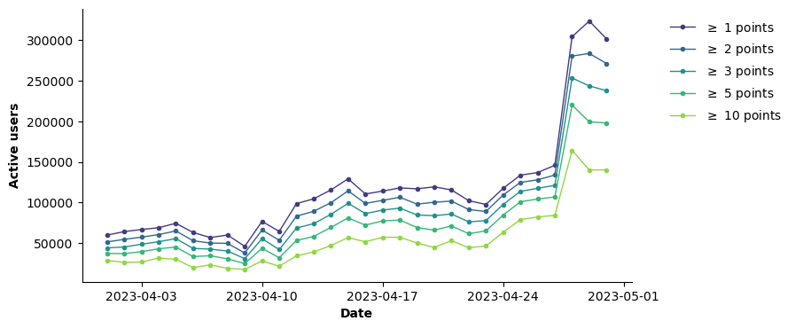
Figure 3. Daily number of active users retained under different minimum points-per-day thresholds (\(\geq\) 1,2,3,5, and 10 points). Increasing the threshold progressively removes low-activity users, reducing sharp spikes driven by users with only one or very few daily points, while preserving temporal trends.

2. Methods

The analysis follows the methodological framework described in Methodological Framework and applied in the previous case study. In brief, we use the Urban Space Usage Index (\(I\)), defined as the share of unique users visiting each H3 hexagon. The number of unique users is used as a proxy for human presence, under the assumption that higher user counts correspond to greater spatial utilization.

To quantify deviations from typical conditions, we compute Z-scores, which measure how strongly observed activity deviates from baseline levels. Positive values indicate higher activity, while negative values indicate lower activity compared to baseline conditions.

3. Results

3.1 Temporal evolution of urban activity

The temporal evolution of the Urban Space Usage Index (\(I\)) shows relatively stable activity levels during the baseline period (April 3-11), with moderate day-to-day variability (Figure 4). A distinct increase in activity is observed between April 12 and 19 (highlighted in red), indicating a temporary deviation from typical conditions. To ensure a stable and representative baseline, we exclude this period, as the elevated activity levels, likely driven by specific events, would bias the reference distribution and inflate Z-score magnitudes. A clear decrease in activity is observed on the first heatwave day (April 20), when activity drops below the baseline average. All heatwave days (marked as red stars) are associated with below-average activity levels, indicating a consistent reduction in urban space usage during periods of extreme heat.

Interestingly, activity remains suppressed not only during heatwave days but also in the intervening days between close heatwave events. While partial recovery is observed on non-heatwave days, activity levels generally remain below or close to the baseline mean.

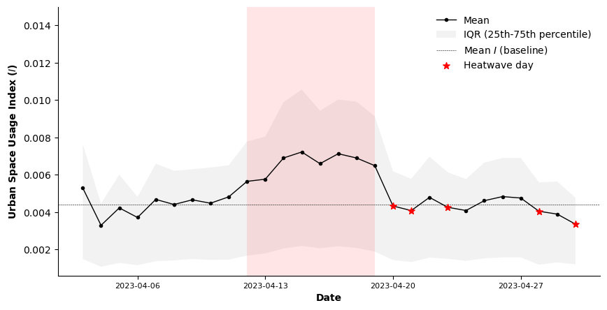
Figure 4. Time series of the median Urban Space Usage Index (\(I\)) across all hexagonal cells in the area of interest, with the shaded area representing the interquartile range. Red stars indicate heatwave days, while the shaded red area represents the period excluded from the baseline.

3.2 Anomaly detection

To assess whether observed changes correspond to statistically significant deviations from typical conditions, we use the Z-score, which measures how many standard deviations observed activity deviates from its baseline.

During the baseline period, Z-scores exhibit some variability, with slightly negative values in the early days followed by stabilization closer to zero (Figure 5). This reflects moderate fluctuations in activity even under typical conditions.

Among the five heatwave days, three exhibit negative Z-scores (-0.20, -0.41, and -0.79 for April 21, 28, and 30, respectively), indicating reduced activity relative to baseline levels. The remaining two days show small positive deviations (0.13 and 0.30 for April 20 and 23, respectively), suggesting that the overall impact on aggregate activity is limited in magnitude.

On average, heatwave days have a Z-score of -0.19, compared to 0.40 for non-heatwave days in the same post-baseline period. To assess whether this difference is statistically significant, we compare heatwave and non-heatwave days from April 20 onward. We test the null hypothesis (\(H_0\)) that both sets of days are drawn from the same distribution, against the alternative hypothesis (\(H_1\)) that heatwave days exhibit lower Z-scores, using a significance level of \(\alpha = 0.05\).

A one-sided Mann-Whitney U test indicates that heatwave days have significantly lower Z-scores than non-heatwave days (p = 0.041). This result is further supported by an exact permutation test, which compares the observed mean Z-score of heatwave days against all possible combinations of five days from the same sample (p = 0.03).

These results suggest that heatwave conditions are associated with a systematic but modest reduction in activity relative to contemporaneous non-heatwave days, consistent with their nature as non-disruptive events. Sensitivity analysis using alternative baseline periods yields consistent results, with similar Mann–Whitney and permutation test outcomes, confirming that the observed reduction is robust to baseline selection.

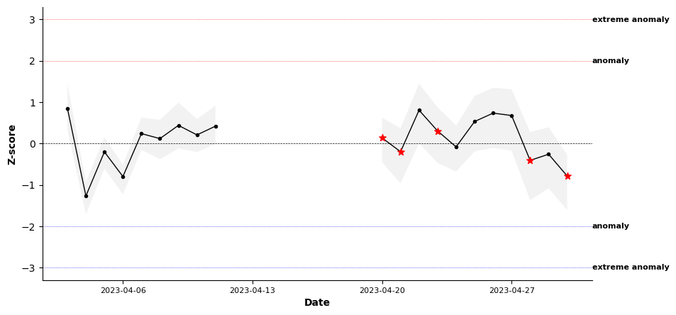
Figure 5. Time series of the average Z-score of the Urban Space Usage Index across hexagons in Metro Manila, with the shaded area representing the interquartile range. Horizontal dashed lines indicate anomaly thresholds. The missing segment corresponds to observations excluded from the baseline due to elevated activity.

3.3 Spatial distribution of anomalies

The spatial distribution of Z-scores during 21 April (Figure 6) does not reveal strong large-scale patterns of activity change. Instead, deviations from baseline are relatively diffuse, with a slight predominance of negative values and clusters of higher and lower activity. This suggests that, unlike disruptive events which often produce clear spatial concentrations of activity, heatwaves do not induce a uniform or city-wide reorganization of urban dynamics.

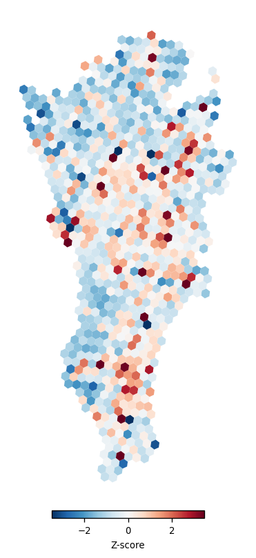
Figure 6. Map of the Z-score of the Urban Space Usage Index across H3 hexagonal cells in Metro Manila on 30 April 2023. Warmer colors indicate higher-than-expected activity.

We also provide an interactive map (Figure 7) to facilitate exploration of the full time series of Z-scores across the study area. This tool enables users to examine temporal dynamics at different locations, offering a more detailed and intuitive understanding of how activity patterns evolve over time.

Make this Notebook Trusted to load map: File -> Trust Notebook

Figure 7. Interactive map of the Z-score of the Urban Space Usage Index across H3 hexagonal cells in the area of interest. The animation shows the day-by-day evolution of activity levels, with colors indicating relative intensity.

3.4 Spatial and Functional Characterization of Activity

To interpret the spatial distribution of activity, each hexagonal cell is associated with both land use and functional activity. For land use, we assign each hexagon a dominant category (e.g., residential, commercial, industrial, green areas), capturing the physical organization of urban space. In contrast, the functional layer is derived from POIs: for each hexagon, we count the number of POIs in different activity categories (e.g., schools, hospitals, parks, transport hubs, commercial venues). For more details on the land use and functional activity methodology, refer to Spatial Characterization of Urban Units.

Land-use and POI data are derived from OpenStreetMap (OSM) and accessed via Geofabrik extracts (https://download.geofabrik.de/asia/philippines.html). To ensure temporal consistency with the mobility data, which refer to 2023, we use OSM snapshots from January 2023. © OpenStreetMap contributors, licensed under the Open Database License (ODbL).

Land Use Analysis

We analyze how urban activity is distributed across different land-use categories during heatwave days, considering both aggregate patterns and day-specific variations.

At the aggregate level, the results show a heterogeneous response across land-use types. Commercial and green areas exhibit positive average Z-scores (0.19 and 0.40, respectively), indicating slightly higher activity relative to baseline levels. In contrast, construction (-0.69), water (-0.47), residential (-0.19), industrial (-0.17), and farmland (-0.22) areas show negative Z-scores, reflecting reduced activity.

These patterns suggest a shift in activity toward specific types of environments during heatwave conditions. In particular, the increase in commercial areas may reflect a preference for indoor, climate-controlled spaces, while the positive signal in green areas may be associated with their role as relatively cooler or shaded environments. Conversely, the decline in construction and industrial areas likely reflects reduced activity in outdoor settings, which are more exposed to extreme heat.

Land Use	Z-score (event)	I (event)	I (baseline)
commercial	0.19	0.00788	0.00784
green	0.40	0.00537	0.00518
construction	-0.69	0.00432	0.00508
residential	-0.19	0.00395	0.00428
water	-0.47	0.00284	0.00362
industrial	-0.17	0.00304	0.00359
farmland	-0.22	0.00047	0.00050

A day-by-day analysis reveals additional variability across heatwave events (see Figure 8). Early heatwave days (April 20-23) are characterized by positive or near-neutral Z-scores in commercial and green areas, while later events (April 28 and 30) show a more generalized decline across most land-use categories.

	Z-score (all)	Z-score (04-20)	Z-score (04-21)	Z-score (04-23)	Z-score (04-28)	Z-score (04-30)
commercial	0.19	0.53	0.50	0.27	0.66	-0.99
construction	-0.69	-0.23	-1.02	-0.13	-0.94	-1.15
farmland	-0.22	0.19	-0.27	0.79	-1.03	-0.80
green	0.40	0.64	0.68	0.29	0.90	-0.49
industrial	-0.17	0.05	-0.16	0.10	-0.13	-0.73
residential	-0.19	0.16	-0.21	0.40	-0.55	-0.73
water	-0.47	-0.16	-0.59	0.06	-0.69	-0.95

Overall, while aggregate activity levels remain relatively stable, heatwave conditions are associated with a redistribution of activity across land-use types. This supports the interpretation that individuals adapt to extreme heat not by substantially reducing mobility, but by shifting their activities toward more suitable areas.

Loading BokehJS ...

Figure 8. Time series of the average Z-score of the Urban Space Usage Index for different land-use classes, with horizontal dashed lines indicating anomaly thresholds.

Functional (POI-Based) Analysis

We then examine activity across functional layers derived from points of interest (POIs), capturing how different types of urban services and destinations are affected by heatwaves. At the aggregate level, most categories exhibit negative Z-scores, indicating a reduction in activity relative to the baseline. The largest decreases are observed for airports (-1.06), highways (-0.50), train stations (-0.43), and universities (-0.39). Other categories, including hospitals (-0.32), tourism (-0.28), restaurants (-0.24), shops (-0.25), schools (-0.25), and offices (-0.21), also show moderate decreases.

In contrast, malls (0.11) and parks (0.14) exhibit slightly positive Z-scores, indicating stable or marginally increased activity during heatwave days. These patterns suggest a shift toward specific types of environments under extreme heat conditions. The increase in mall-related activity may reflect a preference for indoor and climate-controlled spaces, while parks may serve as relatively cooler or shaded areas.

POI layer	Z-score (event)	I (event)	I (baseline)
train stations	-0.43	0.00864	0.00948
malls	0.11	0.00798	0.00806
universities	-0.39	0.00680	0.00728
parks	0.14	0.00751	0.00725
tourism	-0.28	0.00640	0.00704
highways	-0.50	0.00607	0.00696
hospitals	-0.32	0.00546	0.00588
offices	-0.21	0.00522	0.00569
restaurants	-0.24	0.00505	0.00549
schools	-0.25	0.00484	0.00523
airports	-1.06	0.00357	0.00494
shops	-0.25	0.00453	0.00494

The day-by-day analysis reveals consistent patterns across events (see Figure 9). Early heatwave days (April 20-23) show slightly positive deviations for several categories, including malls and parks. However, later heatwave days (April 28 and 30) are associated with a more pronounced decline across nearly all categories, including those that previously showed resilience.

	Z-score (all)	Z-score (04-20)	Z-score (04-21)	Z-score (04-23)	Z-score (04-28)	Z-score (04-30)
highways	-0.50	-0.08	-0.61	0.06	-0.65	-1.23
airports	-1.06	-0.66	-1.09	-0.89	-0.87	-1.80
hospitals	-0.32	0.05	-0.24	0.14	-0.42	-1.13
malls	0.11	0.29	0.30	0.28	0.48	-0.81
offices	-0.21	0.12	-0.14	0.16	-0.24	-0.96
restaurants	-0.24	0.09	-0.22	0.19	-0.35	-0.92
schools	-0.25	0.12	-0.25	0.22	-0.40	-0.93
shops	-0.25	0.10	-0.25	0.23	-0.42	-0.91
tourism	-0.28	0.11	-0.19	0.00	-0.21	-1.12
train stations	-0.43	0.06	-0.43	-0.20	-0.24	-1.35
universities	-0.39	-0.06	-0.29	-0.15	-0.06	-1.39
parks	0.14	0.64	0.59	-0.07	0.68	-1.16

Overall, the results reinforce the findings from the land-use analysis: while aggregate activity levels remain relatively stable, heatwave conditions lead to a redistribution of activity toward environments that are more compatible with extreme heat exposure.

Figure 9. Time series of the average Z-score of the Urban Space Usage Index for different functional layers, with horizontal dashed lines indicating anomaly thresholds.

4. Conclusions and Key Findings

This analysis quantifies the impact of heatwaves on urban activity patterns in Metro Manila using anonymized mobility data and the Urban Space Usage Index.

The main findings are:

1. Aggregate activity levels remain relatively stable during heatwave days, with only modest deviations from baseline conditions. Z-scores are generally close to zero, with three out of five heatwave days exhibiting negative values, and an overall slight but statistically significant reduction compared to non-heatwave days.

2. Heatwaves induce a redistribution of activity rather than large aggregate changes. While overall activity levels are only marginally affected, land-use and POI-based analyses reveal systematic shifts in how urban space is used.

3. Activity shifts toward environments more compatible with extreme heat exposure. In particular, commercial areas and malls show stable or slightly increased activity, as do green areas, potentially reflecting their role as relatively cooler or shaded environments.

4. Heatwaves exhibit a distinct impact compared to other types of events. While large planned events (e.g., Republic Day) and sudden shocks (e.g., earthquakes) produce strong and immediate changes in both aggregate activity and spatial visitation patterns, heatwaves generate a weaker aggregate signal but a clear pattern of spatial and functional redistribution.

Overall, these results suggest that while the proposed framework and the Urban Space Usage Index may not detect strong anomalies for heatwaves at the aggregate level, it is well suited to uncovering underlying patterns of spatial and functional redistribution.

Policy relevance

This analysis can support urban heat adaptation and climate resilience planning by showing how activity changes during periods of extreme heat. For the 2023 heatwaves in Metro Manila, the results indicate that aggregate activity remains relatively stable, but urban space usage shifts across land-use and functional categories. In particular, activity is lower in more exposed outdoor or infrastructure-related areas and remains stable or slightly higher in commercial areas, malls, and green spaces. These results can inform the planning of cooling centers, shaded public spaces, and targeted interventions in areas where people continue to concentrate during extreme heat.

Limitations

This analysis is subject to some limitations. Mobility data may not fully represent the entire population, as it depends on smartphone usage and data coverage. In addition, spatial aggregation into H3 cells may smooth local variations.