Chapter 5 Cleaning and processing research data

Original data come in a variety of formats, most of which are not immediately suited for analysis. The process of preparing data for analysis has many different names—data cleaning, data munging, data wrangling—but they all mean the same thing: transforming data into an appropriate format for the intended use. This task is the most time-consuming step of a project’s data work, particularly when primary data are involved; it is also critical for data quality. A structured workflow for preparing newly acquired data for analysis is essential for efficient, transparent, and reproducible data work. A key point of this chapter is that no changes are made to the contents of data at this point. Therefore, the clean data set, which is the main output from the workflow discussed in this chapter, contains the same information as the original data, but in a format that is ready for use with statistical software. Chapter 6 discusses tasks that involve changes to the data based on research decisions, such as creating new variables, imputing values, and handling outliers.

This chapter describes the various tasks involved in making newly acquired data ready for analysis. The first section teaches how to make data tidy, which means adjusting the organization of the data set until the relationship between rows and columns is well defined. The second section describes quality assurance checks, which are necessary to verify data accuracy. The third section covers de-identification, because removing direct identifiers early in the data-handling process helps to ensure privacy. The final section discusses how to examine each variable in the data set and ensure that it is as well documented and as easy to use as possible. Each of these tasks is implemented through code, and the resulting data sets can be reproduced exactly by running this code. The original data files are kept precisely as they were acquired, and no changes are made directly to them. Box 5.1 summarizes the main points, lists the responsibilities of different members of the research team, and supplies a list of key tools and resources for implementing the recommended practices.

BOX 5.1 SUMMARY: CLEANING AND PROCESSING RESEARCH DATA

After being acquired, data must be structured for analysis in accordance with the research design, as laid out in the data linkage tables and the data flowcharts discussed in chapter 3. This process entails the following tasks.

1.Tidy the data. Many data sets do not have an unambiguous identifier as received, and the rows in the data set often do not match the units of observation specified by the research plan and data linkage table. To prepare the data for analysis requires two steps:

Determine the unique identifier for each unit of observation in the data.
Transform the data so that the desired unit of observation uniquely identifies rows in each data set.

2.Validate data quality. Data completeness and quality should be validated upon receipt to ensure that the information is an accurate representation of the characteristics and individuals it is supposed to describe. This process entails three steps:

Check that the data are complete—that is, that all the observations in the desired sample were received.
Make sure that data points are consistent across variables and data sets.
Explore the distribution of key variables to identify outliers and other unexpected patterns.

3.De-identify, correct, and annotate the data. After the data have been processed and de-identified, the information must be archived, published, or both. Before publication, it is necessary to ensure that the processed version is highly accurate and appropriately protects the privacy of individuals:

De-identify the data in accordance with best practices and relevant privacy regulations.
Correct data points that are identified as being in error compared to ground reality.
Recode, document, and annotate data sets so that all of the content will be fully interpretable by future users, whether or not they were involved in the acquisition process.

Key responsibilities for task team leaders and principal investigators

Determine the units of observation needed for experimental design and supervise the development of appropriate unique identifiers.
Indicate priorities for quality checks, including key indicators and reference values.
Provide guidance on how to resolve all issues identified in data processing, cleaning, and preparation.
Publish or archive the prepared data set.

Key responsibilities for research assistants

Develop code, data, and documentation linking data sets with the data map and study design, and tidy all data sets to correspond to the required units of observation.
Manage data quality checks, and communicate issues clearly to task team leaders, principal investigators, data producers, and field teams.
Inspect each variable, recoding and annotating as required. Prepare the data set for publication by de-identifying data, correcting field errors, and documenting the data.

Key Resources

The iefieldkit Stata package, a suite of commands to enable reproducible data cleaning and processing:.
- Explanation at https://dimewiki.worldbank.org/iefieldkit
- codetools at https://github.com/worldbank/iefieldkit
The ietoolkit Stata package, a suite of commands to enable reproducible data management and analysis:.
- Explanation at https://dimewiki.worldbank.org/ietoolkit
- Code at https://github.com/worldbank/ietoolkit
DIME Analytics Continuing Education Session on Tidying Data at https://osf.io/p4e8u/
De-identification article on DIME Wiki at https://dimewiki.worldbank.org/De-identification

Making data “tidy”

The first step in creating an analysis data set is to understand the data acquired and use this understanding to translate the data into an intuitive format. This section discusses what steps may be needed to make sure that each row in a data table⁷⁷ represents one observation. Getting to such a format may be harder than expected, and the unit of observation⁷⁸ may be ambiguous in many data sets. This section presents the tidy data format, which is the ideal format for handling tabular data. Tidying data is the first step in data cleaning; quality assurance is best done using tidied data, because the relationship between row and unit of observation is as simple as possible. In practice, tidying and quality monitoring should proceed simultaneously as data are received.

This book uses the term “original data” to refer to the data in the state in which the information was first acquired by the research team. In other sources, the terms “original data” or “raw data” may be used to refer to the corrected and compiled data set created from received information, which this book calls “clean data”—that is, data that have been processed to have errors and duplicates removed, that have been transformed to the correct level of observation, and that include complete metadata such as labels and documentation. This phrasing applies to data provided by partners as well as to original data collected by the research team.

Establishing a unique identifier

Before starting to tidy a data set, it is necessary to understand the unit of observation that the data represent and to determine which variable or set of variables is the unique identifier⁷⁹ for each observation. As discussed in chapter 3, the unique identifier will be used to link observations in this data set to data in other data sources according to the data linkage table⁸⁰, and it must be listed in the master data set⁸¹

Ensuring that observations are uniquely and fully identified is arguably the most important step in data cleaning because the ability to tidy the data and link them to any other data sets depends on it. It is possible that the variables expected to identify the data uniquely contain either missing or duplicate values in the original data. It is also possible that a data set does not include a unique identifier or that the original unique identifier is not a suitable project identifier⁸² (ID). Suitable project IDs should not, for example, involve long strings that are difficult to work with, such as names, or be known outside of the research team.

In such cases, cleaning begins by adding a project ID to the acquired data. If a project ID already exists for this unit of observation, then it should be merged carefully from the master data set to the acquired data using other identifying information. (In R and some other languages, this operation is called a “data set join”; this book uses the term “merge.”) If a project ID does not exist, then it is necessary to generate one, add it to the master data set, and then merge it back into the original data. Although digital survey tools create unique identifiers for each data submission, these identifiers are not the same as having a unique ID variable for each observation in the sample, because the same observation can have multiple submissions.

The DIME Analytics team created an automated workflow to identify, correct, and document duplicated entries in the unique identifier using the ieduplicates⁸³ and iecompdup⁸⁴ Stata commands. One advantage of using ieduplicates to correct duplicate entries is that it creates a duplicates report, which records each correction made and documents the reason for it. Whether using this command or not, it is important to keep a record of all cases of duplicate IDs encountered and how they were resolved (see box 5.2 for an explanation of how a unique identifier was established for the Demand for Safe Spaces project).

BOX 5.2 ESTABLISHING A UNIQUE IDENTIFIER: A CASE STUDY FROM THE DEMAND FOR SAFE SPACES PROJECT

All data sets have a unit of observation, and the first columns of each data set should uniquely identify which unit is being observed. In the Demand for Safe Spaces project, as should be the case in all projects, the first few lines of code that imported each original data set immediately ensured that this was true and applied any corrections from the field needed to fix errors related to uniqueness.

The code segment below was used to import the crowdsourced ride data; it used the ieduplicates command to remove duplicate values of the uniquely identifying variable in the data set. The screen shot of the corresponding ieduplicates report shows how the command documents and resolves duplicate identifiers in data collection. After applying the corrections, the code confirms that the data are uniquely identified by riders and ride identifiers and documents the decisions in an optimized format.

// Import to Stata format ======================================================

  import delimited using "${encrypt}/Baseline/07112016/Contributions 07112016", ///
      delim(",")         ///
      bindquotes(strict) ///
      varnames(1)        ///
      clear

  * There are two duplicated values for obs_uid, each with two submissions.
  * All four entries are demographic survey from the same user, who seems to
  * have submitted the data twice, each time creating two entries.
  * Possibly a connectivity issue
  ieduplicates obs_uid using "${doc_rider}/baseline-study/raw-duplicates.xlsx", ///
      uniquevars(v1) ///
      keepvars(created submitted started)

  * Verify unique identifier, sort, optimize storage, 
  * remove blank entries and save data
  isid user_uuid obs_uid, sort
  compress
  dropmiss, force
  save             "${encrypt}/baseline_raw.dta", replace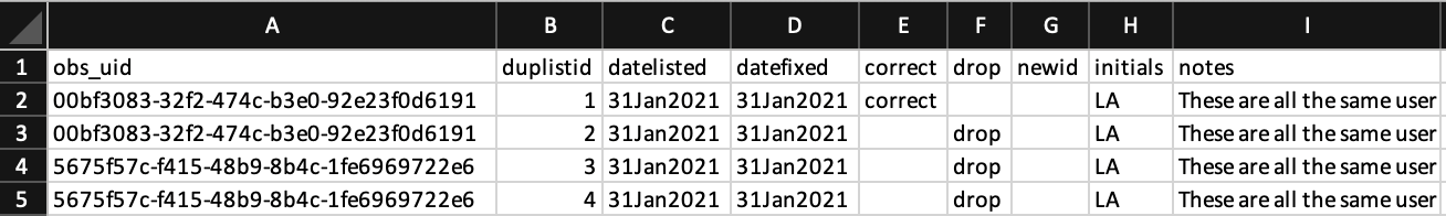

To access this code in do-file format, visit the GitHub repository at https://github.com/worldbank/dime-data-handbook/tree/main/code.

Tidying data

Although data can be acquired in all shapes and sizes, they are most commonly received as one or multiple data tables. These data tables can organize information in multiple ways, and not all of them result in easy-to-handle data sets. Fortunately, a vast literature of database management has identified the format that makes interacting with the data as easy as possible. While this is called normalization in database management, data in this format are called tidy in data science. A data table is tidy when each column represents one variable⁸⁵, each row represents one observation⁸⁶, and all variables in it have the same unit of observation. Every other format is untidy. This distinction may seem trivial, but data, and original survey data in particular, are rarely received in a tidy format.

The most common case of untidy data acquired in development research is a data set with multiple units of observations stored in the same data table. When the rows include multiple nested observational units, then the unique identifier does not identify all observations in that row, because more than one unit of observation is in the same row. Survey data containing nested units of observation are typically imported from survey platforms in wide format⁸⁷. Wide format data could have, for instance, one column for a household-level variable (for example, owns_fridge) and a few columns for household member–level variables (for example, sex_1, sex_2). Original data are often saved in this format because it is an efficient way to transfer the data: adding different levels of observation to the same data table allows data to be transferred in a single file. However, doing so leads to the widespread practice of interacting with data in wide format, which is often inefficient and error-prone.

To understand how dealing with wide data can be complicated, imagine that the project needs to calculate the share of women in each household. In a wide data table, it is necessary first to create variables counting the number of women and the total number of household members and then to calculate the share; otherwise, the data have to be transformed to a different format. In a tidy data table, however, in which each row is a household member, it is possible to aggregate the share of women by household, without taking additional steps, and then to merge the result to the household-level data tables. Tidy data tables are also easier to clean, because each attribute corresponds to a single column that needs to be checked only once, and each column corresponds directly to one question in the questionnaire. Finally, summary statistics and distributions are much simpler to generate from tidy data tables.

As mentioned earlier, there are unlimited ways for data to be untidy; wide format is only one of those ways. Another example is a data table containing both information on transactions and information on the firms involved in each transaction. In this case, the firm-level information is repeated for all transactions in which a given firm is involved. Analyzing firm data in this format gives more weight to firms that conducted more transactions, which may not be consistent with the research design.

The basic process behind tidying a data table is simple: first, identify all of the variables that were measured at the same level of observation; second, create separate data tables for each level of observation; and third, reshape⁸⁸ the data and remove duplicate rows until each data table is uniquely and fully identified by the unique identifier that corresponds to its unit of observation. Reshaping data tables is one of the most intricate tasks in data cleaning. It is necessary to be very familiar with commands such as reshape in Stata and pivot in R. It is also necessary to ensure that identifying variables are consistent across data tables, so they can always be linked. Reshaping is the type of transformation referred to in the example of how to calculate the share of women in a wide data set. The important difference is that in a tidy workflow, instead of reshaping the data for each operation, each such transformation is done once during cleaning, making all subsequent operations much easier.

In the earlier household survey example, household-level variables are stored in one tidy data table, and household-member variables are reshaped and stored in a separate, member-level, tidy data table, which also contains the household ID for each individual. The household ID is intentionally duplicated in the household-member data table to allow one or several household members to be linked to the same household data. The unique identifier for the household member–level data will be either a single household member ID or a combination of household ID and household member ID. In the transaction data example, the tidying process creates one transaction-level data table, containing variables indicating the ID of all firms involved, and one firm-level data table, with a single entry for each firm. Then, firm-level analysis can be done easily by calculating appropriate statistics in the transactions data table (in Stata, often through collapse) and then merging or joining those results with the firm data table.

In a tidy workflow, the clean data set contains one or more tidy data tables (see box 5.3 for an example of how data sets were tidied in the Demand for Safe Spaces project). In both examples in the preceding paragraphs, the clean data set is made up of two tidy data tables. There must be a clear way to connect each tidy data table to a master data set and thereby also to all other data sets. To implement this connection, one data table is designated as the main data table, and that data table’s unit of observation is the main unit of observation of the data set. It is important that the main unit of observation correspond directly to a master data set and be listed in the data linkage table. There must be an unambiguous way to merge all other data tables in the data set with the main data table. This process makes it possible to link all data points in all of the project’s data sets to each other. Saving each data set as a folder of data tables, rather than as a single file, is recommended: the main data table shares the same name as the folder, and the names of all other data tables start with the same name, but are suffixed with the unit of observation for that data table.

BOX 5.3 TIDYING DATA: A CASE STUDY FROM THE DEMAND FOR SAFE SPACES PROJECT

The unit of observation in an original data set does not always match the relevant unit of analysis for a study. One of the first steps required is to create data sets at the unit of analysis desired. In the case of the crowdsourced ride data used in the Demand for Safe Spaces project, study participants were asked to complete three tasks in each metro trip: one before boarding the train (check-in task), one during the ride (ride task), and one after leaving the train (check-out task). The raw data sets show one task per row. As a result, each unit of analysis, a metro trip, was described in three rows in this data set.

To create a data set at the trip level, the research team took two steps, outlined in the data flowchart (for an example of how data flowcharts can be created, see box 3.3 in chapter 3). First, three separate data sets were created, one for each task, containing only the variables and observations created during that task. Then the trip-level data set was created by combining the variables in the data tables for each task at the level of the individual trip (identified by the session variable).

The following code shows an example of the ride task script, which keeps only the ride task rows and columns from the raw data set.

/*******************************************************************************
    Load data set and keep ride variables
*******************************************************************************/

    use "${dt_raw}/baseline_raw_deidentified.dta", clear

    * Keep  only entries that refer to ride task
    keep if inlist(spectranslated, "Regular Car", "Women Only Car")

    * Sort observations
    isid user_uuid session, sort

    * Keep only questions answered during this task
    * (all others will be missing for these observations)
    dropmiss, force

The script then encodes categorical variables and saves a tidy ride task data set:

/*******************************************************************************
    Clean up and save
*******************************************************************************/

    iecodebook apply using "${doc_rider}/baseline-study/codebooks/ride.xlsx", drop
    order  user_uuid session RI_pa - RI_police_present CI_top_car RI_look_pink ///
           RI_look_mixed RI_crowd_rate RI_men_present
  
    * Optimize memory and save data
    compress
    save "${dt_int}/baseline_ride.dta", replace

The same procedure was repeated for the check-in and check-out tasks. Each of these tidy data sets was saved with a very descriptive name, indicating the wave of data collection and the task included in the data set. For the complete script, visit the GitHub repository at https://git.io/Jtgqj.

In the household data set example, the household-level data table is the main table. This means that there must be a master data set for households. (The project may also have a master data set for household members if it is important for the research, but having one is not strictly required.) The household data set would then be stored in a folder called, for example, baseline-hh-survey. That folder would contain both the household-level data table with the same name as the folder, for example, baseline-hh-survey.csv, and the household member– level data, named in the same format but with a suffix, for example, baseline-hh-survey-hhmember.csv.

The tidying process gets more complex as the number of nested groups increases. The steps for identifying the unit of observation of each variable and reshaping the separated data tables need to be repeated multiple times. However, the larger the number of nested groups in a data set, the more efficient it is to deal with tidy data than with untidy data. Cleaning and analyzing wide data sets, in particular, constitute a repetitive and error-prone process.

The next step of data cleaning—data quality monitoring—may involve comparing different units of observation. Aggregating subunits to compare to a higher unit is much easier with tidy data, which is why tidying data is the first step in the data cleaning workflow. When collecting primary data, it is possible to start preparing or coding the data tidying even before the data are acquired, because the exact format in which the data will be received is known in advance. Preparing the data for analysis, the last task in this chapter, is much simpler when tidying has been done.

Implementing data quality checks

Whether receiving data from a partner or collecting data directly, it is important to make sure that data faithfully reflect realities on the ground. It is necessary to examine carefully any data collected through surveys or received from partners. Reviewing original data will inevitably reveal errors, ambiguities, and data entry mistakes, such as typos and inconsistent values. The key aspects to keep in mind are the completeness, consistency, and distribution of data (Andrade et al. 2021). Data quality assurance checks⁸⁹ should be performed as soon as the data are acquired. When data are being collected and transferred to the team in real time, conducting high-frequency checks⁹⁰ is recommended. Primary data require paying extra attention to quality checks, because data entry by humans is susceptible to errors, and the research team is the only line of defense between data issues and data analysis. Chapter 4 discusses survey-specific quality monitoring protocols.

Data quality checks should carefully inspect key treatment and outcome variables to ensure that the data quality of core study variables is uniformly high and that additional effort is centered where it is most important. Checks should be run every time data are received to flag irregularities in the acquisition progress, in sample completeness, or in response quality. The faster issues are identified, the more likely they are to be solved. Once the field team has left a survey area or high-frequency data have been deleted from a server, it may be impossible to verify whether data points are correct or not. Even if the research team is not receiving data in real time, the data owners may not be as knowledgeable about the data or as responsive to the research team queries as time goes by. ipacheck is a very useful Stata command that automates some of these tasks, regardless of the data source.

It is important to check continuously that the observations in data match the intended sample. In surveys, electronic survey software often provides case management features through which sampled units are assigned directly to individual enumerators. For data received from partners, such as administrative data, this assignment may be harder to validate. In these cases, cross-referencing with other data sources can help to ensure completeness. It is often the case that the data as originally acquired include duplicate observations⁹¹ or missing entries, which may occur because of typos, failed submissions to data servers, or other mistakes. Issues with data transmission often result in missing observations, particularly when large data sets are being transferred or when data are being collected in locations with limited internet connection. Keeping a record of what data were submitted and then comparing it to the data received as soon as transmission is complete reduces the risk of noticing that data are missing when it is no longer possible to recover the information.

Once data completeness has been confirmed, observed units must be validated against the expected sample: this process is as straightforward as merging the sample list with the data received and checking for mismatches. Reporting errors and duplicate observations in real time allows for efficient corrections. ieduplicates provides a workflow for resolving duplicate entries with the data provider. For surveys, it is also important to track the progress of data collection to monitor attrition, so that it is known early on if a change in protocols or additional tracking is needed (for an example, Özler et al. (2016)). It is also necessary to check survey completion rates and sample compliance by surveyors and survey teams, to compare data missingness across administrative regions, and to identify any clusters that may be providing data of suspect quality.

Quality checks should also include checks of the quality and consistency of responses. For example, it is important to check whether the values for each variable fall within the expected range and whether related variables contradict each other. Electronic data collection systems often incorporate many quality control features, such as range restrictions and logical flows. Data received from systems that do not include such controls should be checked more carefully. Consistency checks are project specific, so it is difficult to provide general guidance. Having detailed knowledge of the variables in the data set and carefully examining the analysis plan are the best ways to prepare. Examples of inconsistencies in survey data include cases in which a household reports having cultivated a plot in one module but does not list any cultivated crops in another. Response consistency should be checked across all data sets, because this task is much harder to automate. For example, if two sets of administrative records are received, one with hospital-level information and one with data on each medical staff member, the number of entries in the second set of entries should match the number of employed personnel in the first set.

Finally, no amount of preprogrammed checks can replace actually looking at the data. Of course, that does not mean checking each data point; it does mean plotting and tabulating distributions for the main variables of interest. Doing so will help to identify outliers and other potentially problematic patterns that were not foreseen. A common source of outlier values in survey data are typos, but outliers can also occur in administrative data if, for example, the unit reported changed over time, but the data were stored with the same variable name. Identifying unforeseen patterns in the distribution will also help the team to gather relevant information—for example, if there were no harvest data because of a particular pest in the community or if the unusual call records in a particular area were caused by temporary downtime of a tower. Analysis of metadata can also be useful in assessing data quality. For example, electronic survey software generates automatically collected timestamps and trace histories, showing when data were submitted, how long enumerators spent on each question, and how many times answers were changed before or after the data were submitted. See box 5.4 for examples of data quality checks implemented in the Demand for Safe Spaces project.

BOX 5.4 ASSURING DATA QUALITY: A CASE STUDY FROM THE DEMAND FOR SAFE SPACES PROJECT

The Demand for Safe Spaces team adopted three categories of data quality assurance checks for the crowdsourced ride data. The first—completeness—made sure that each data point made technical sense in that it contained the right elements and that the data as a whole covered all of the expected spaces. The second—consistency—made sure that real-world details were right: stations were on the right line, payments matched the value of a task, and so on. The third—distribution—produced visual descriptions of the key variables of interest to make sure that any unexpected patterns were investigated further. The following are examples of the specific checks implemented:

Completeness

Include the following tasks in each trip: check-in, ride, and check-out.
Plot the number of observations per day of the week and per half-hour time-bin to make sure that there are no gaps in data delivery.
Plot all observations received from each combination of line and station to visualize data coverage.

Consistency

Check the correspondence between stations and lines. This check identified mismatches that were caused by the submission of lines outside the research sample. These observations were excluded from the corrected data.
Check the correspondence between task and premium for riding in the women-only car. This check identified a bug in the app that caused some riders to be offered the wrong premium for some tasks. These observations were excluded from the corrected data.
Check task times to make sure they were applied in the right order. The task to be completed before boarding the train came first, then the one corresponding to the trip, and finally the one corresponding to leaving the station.

Distribution

Compare platform observations data and rider reports of crowding and male presence to ensure general data agreement.
Visualize distribution of rides per task per day and week to ensure consistency.
Visualize patterns of the presence of men in the women-only car throughout the network.

Processing confidential data

When implementing the steps discussed up to this point, the team is likely to be handling confidential data. Effective monitoring of data quality frequently requires identifying individual observations in the data set and the people or other entities that the data describe. Using identified data enables rapid follow-up on and resolution of identified issues. Handling confidential data such as personally identifying information⁹² (PII) requires a secure environment and, typically, encryption. De-identifying the data simplifies the workflow and reduces the risk of harmful leaks. This section describes how to de-identify data in order to share the information with a wider audience.

Protecting research subject privacy

Most development data involve human subjects⁹³. Researchers often have access to personal information about people: where they live, how much they earn, whether they have committed or been victims of crimes, their names, their national identity numbers, and other sensitive data (for an example, see A. Banerjee, Ferrara, and Orozco (2019)). There are strict requirements for safely storing and handling personally identifying data, and the research team is responsible for satisfying these requirements. Everyone working with research on human subjects should have completed an ethics certification course, such as Protecting Human Research Participants (https://phrptraining.com) or one of the CITI Program course offerings (https://citiprogram.org). A plan for handling data securely is typically also required for institutional review board (IRB) approval.

The best way to avoid risk is to minimize interaction with PII as much as possible. First, only PII that is strictly necessary for the research should be collected. Second, there should never be more than one copy of any identified data set in the working project folder, and this data set must always be encrypted. Third, data should be de-identified as early as possible in the workflow. Even within the research team, access to identified data should be limited to team members who require it for their specific tasks. Data analysis rarely requires identifying information, and, in most cases, masked identifiers can be linked to research information, such as treatment status and weight, and then unmasked identifiers can be removed.

Once data are acquired and data quality checks have been completed, the next task typically is to de-identify⁹⁴ the data by removing or masking all personally identifying variables. In practice, it is rarely, if ever, possible to anonymize data. There is always some statistical chance that an individual’s identity will be relinked to the project data by using some other data—even if the project data have had all of the directly identifying information removed. For this reason, de-identification should typically be conducted in two stages. The initial de-identification process, performed as soon as data are acquired, strips the data of direct identifiers, creating a working de-identified data set that can be shared within the research team without the need for encryption. The final de-identification process, performed before data are released publicly, involves careful consideration of the trade-offs between the risk of identifying individuals and the utility of the data; it typically requires removing a further level of indirect identifiers. The rest of this section describes how to approach the de-identification process.

Implementing de-identification

Initial de-identification reduces risk and simplifies workflows. Having created a de-identified version of the data set, it is no longer necessary to interact directly with the identified data. If the data tidying has resulted in multiple data tables, each table needs to be de-identified separately, but the workflow will be the same for all of them.

During the initial round of de-identification, data sets must be stripped of directly identifying information. To do so requires identifying all of the variables that contain such information. For data collection, when the research team designs the survey instrument, flagging all potentially identifying variables at the questionnaire design stage simplifies the initial de-identification process. If that was not done or original data were received by another means, a few tools can help to flag variables with directly identifying data. The Abdul Latif Jameel Poverty Action Lab (J-PAL) PII-scan and Innovations for Poverty Action (IPA) PII_detection scan variable names and labels for common string patterns associated with identifying information. The sdcMicro package lists variables that uniquely identify observations, but its more refined method and need for higher processing capacity make it better suited for final de-identification (Benschop and Welch (n.d.)). The iefieldkit command iecodebook⁹⁵ lists all variables in a data set and exports an Excel sheet that makes it easy to select which variables to keep or drop.

It is necessary to assess the resulting list of variables that contain PII against the analysis plan, asking for each variable, Will this variable be needed for the analysis? If not, the variable should be removed from the de-identified data set. It is preferrable to be conservative and remove all identifying information at this stage. It is always possible to include additional variables from the original data set if deemed necessary later. However, it is not possible to go back in time and drop a PII variable that was leaked (see box 5.5 for an example of how de-identification was implemented for the Demand for Safe Spaces project).

BOX 5.5 IMPLEMENTING DE-IDENTIFICATION: A CASE STUDY FROM THE DEMAND FOR SAFE SPACES PROJECT

The Demand for Safe Spaces team used the iecodebook command to drop identifying information from the data sets as they were imported. Additionally, before data sets were published, the labels indicating line and station names were removed from them, leaving only the masked number for the underlying category. This was done so that it would not be possible to reconstruct individuals’ commuting habits directly from the public data.

The code fragment below shows an example of the initial de-identification when the data were imported. The full data set was saved in the folder for confidential data (using World Bank OneDrive accounts), and a short codebook listing variable names, but not their contents, was saved elsewhere. iecodebook was then used with the drop option to remove confidential information from the data set before it was saved in a shared Dropbox folder. The specific variables removed in this operation contained information about the data collection team that was not needed after quality checks were implemented (deviceid, subscriberid, simid, devicephonenum, username, enumerator, enumeratorname) and the phone number of survey respondents (phone_number).

/*******************************************************************************
    PART 4: Save data
*******************************************************************************/

    * Identified version: verify unique identifier, optimize storage, and save data
    isid id, sort
    compress
    save             "${encrypt}/Platform survey/platform_survey_raw.dta", replace

    * De-identify: remove confidential variables only
    iecodebook apply using "${doc_platform}/codebooks/raw_deidentify.xlsx", drop

    * De-identified version: verify unique identifier, optimize storage, and save data
    isid id, sort
    compress
    save             "${dt_raw}/platform_survey_raw_deidentified.dta", replace

For the complete data import do-file, visit the GitHub repository at https://git.io/JtgmU. For the corresponding iecodebook form, visit the GitHub repository at https://git.io/JtgmY.

For each identifying variable that is needed in the analysis, it is necessary to ask, Is it possible to encode or otherwise construct a variable that masks the confidential component and then drop this variable? For example, it is easy to encode identifiers for small localities like villages and provide only a masked numerical indicator showing which observations are in the same village without revealing which villages are included in the data. This process can be done for most identifying information. If the answer to either of the two questions posed is yes, all that needs to be done is to write a script to drop the variables that are not required for analysis, encode or otherwise mask those that are required, and save a working version of the data. For example, after constructing measures of distance or area, drop the specific geolocations in the data; after constructing and verifying numeric identifiers in a social network module, drop all names. If identifying information is strictly required for the analysis and cannot be masked or encoded, then at least the identifying part of the data must remain encrypted and be decrypted only when used during the data analysis process. Using identifying data in the analysis process does not justify storing or sharing the information in an insecure way.

After initial de-identification is complete, the data set will consist of one or multiple tidy, de-identified data tables. This is the data set with which the team will interact during the remaining tasks described in this chapter. Initial de-identification should not affect the usability of the data. Access to the initially de-identified data should still be restricted to the research team only, because indirect identifiers may still present a high risk of disclosure. It is common, and even desirable, for teams to make data publicly available once the tasks discussed in this chapter have been concluded. Making data publicly available will allow other researchers to conduct additional analysis and to reproduce the findings. Before that can be done, however, it is necessary to consider whether the data can be reidentified, in a process called final de-identification, which is discussed in more detail in chapter 7.

Preparing data for analysis

The last step in the process of data cleaning involves making the data set easy to use and understand and carefully examining each variable to document distributions and identify patterns that may bias the analysis. The resulting data set will contain only the variables collected in the field, and data points will not be modified, except to correct mistaken entries. There may be more data tables in the data set now than originally received, and they may be in a different format, but the information contained is still the same. In addition to the cleaned data sets, cleaning will also yield extensive documentation describing the process.

Such detailed examination of each variable yields in-depth understanding of the content and structure of the data. This knowledge is key to correctly constructing and analyzing final indicators, which are covered in the next chapter. Careful inspection of the data is often the most time-consuming task in a project. It is important not to rush through it! This section introduces some concepts and tools to make it more efficient and productive. The discussion is separated into four subtopics: exploring the data, making corrections, recoding and annotating, and documenting data cleaning. They are separated here because they are different in nature and should be kept separate in the code. In practice, however, they all may be done at the same time.

Exploring the data

The first time a project team interacts with the data contents is during quality checks. However, these checks are usually time-sensitive, and there may not be time to explore the data at length. As part of data processing, each variable should be inspected closely. Tabulations, summary statistics, histograms, and density plots are helpful for understanding the structure of data and finding patterns or irregularities. Critical thinking is essential: the numerical values need to be consistent with the information the variable represents. Statistical distributions need to be realistic and not be unreasonably clumped or skewed. Related variables need to be consistent with each other, and outliers and missing values need to be found. If unusual or unexpected distributional patterns are found for any of these characteristics, data entry errors could be the cause.

At this point, it is more important to document the findings than to address any irregularities. A very limited set of changes should be made to the original data set during cleaning. They are described in the next two sections and are usually applied to each variable as it is examined. Most of the transformations that result in new variables occur during data construction⁹⁶, a process discussed in the next chapter. For now, the task is to focus on creating a record of what is observed and to document extensively the data being explored. This documentation is useful during the construction phase when discussing how to address irregularities and also valuable during exploratory data analysis.

Correcting data points

As mentioned earlier, corrections to issues identified during data quality monitoring are the only changes made to individual data points during the data-cleaning stage. However, there is a lot of discussion about whether such data points should be modified at all. On the one hand, some argue that following up on the issues identified is costly and adds limited value. Because it is not possible to check each and every possible data entry error, identifying issues on just a few main variables can create a false sense of security. Additionally, manually inspected data may suffer from considerable inspector variability. In many cases, the main purpose of data quality checks is to detect fraud and identify problems with data collection protocols. On the other hand, others argue against keeping clear errors or not correcting missing values. DIME Analytics recommends correcting any entries that are clearly identified as errors. However, there is some subjectivity involved in deciding which cases fall into this category. A common rule of thumb is to include the set of corrections based on information that the team has privileged access to and other research teams would not be able to make, and no more. Making this decision involves deep knowledge of the data and the particular circumstances of each research project.

Whether the decision is made to modify data or not, it is essential to keep a careful record of all the issues identified. If no data points are modified, it may still be helpful to add flags to observations containing potentially problematic values so that it is possible to verify how they affect results during analysis. If the team decides to follow up on and correct these issues, the follow-up process must be documented thoroughly. Confidential information should never be included in documentation that is not stored securely or that will be released as part of a replication package or data publication. Finally, no changes should be made directly to the original data set. Instead, any corrections must be made as part of data cleaning, applied through code, and saved to a new data set (see box 5.6 for a discussion of how data corrections were made for the Demand for Safe Spaces project).

BOX 5.6 CORRECTING DATA POINTS: A CASE STUDY FROM THE DEMAND FOR SAFE SPACES PROJECT

Most of the issues that the Demand for Safe Spaces team identified in the raw crowdsourced data during data quality assurance were related to incorrect station and line identifiers. Two steps were taken to address this issue. The first was to correct data points. The second was to document the corrections made.

The correct values for the line and station identifiers, as well as notes on how they were identified, were saved in a data set called station_correction.dta. The team used the command merge to replace the values in the raw data in memory (called the “master data” in merge) with the station_correction.dta data (called the “using data” in merge). The following options were used for the following reasons:

update replace was used to update values in the “master data” with values from the same variable in the “using data.”
keepusing(user_station) was used to keep only the user_station variable from the “using data.”
assert(master match_update) was used to confirm that all observations were either only in the “master data” or were in both the “master data” and the “using data” and that the values were updated with the values in the “using data.” This quality assurance check was important to ensure that data were merged as expected.

To document the final contents of the original data, the team published supplemental materials on GitHub as well as on the World Bank Microdata Catalog.

* There was a problem with the line option for one of the stations.
* This fixes it:
* --------------------------------------------------------------------

    merge 1:1 obs_uuid                                               ///
      using "${doc_rider}/compliance-pilot/station_corrections.dta", ///
      update replace                                                 ///
      keepusing(user_station)                                        ///
      assert(master match_update)                                    ///
      nogen

For the complete script, visit the GitHub repository at https://git.io/Jt2ZC.

Recoding and annotating data

The clean data set is the starting point of data analysis. It is manipulated extensively to construct analysis indicators, so it must be easy to process using statistical software. To make the analysis process smoother, the data set should have all of the information needed to interact with it. Having this information will save people opening the data set from having to go back and forth between the data set and its accompanying documentation, even if they are opening the data set for the first time.

Often, data sets are not imported into statistical software in the most efficient format. The most common example is string (text) variables: categorical variables⁹⁷ and open-ended responses are often read as strings. However, variables in this format cannot be used for quantitative analysis. Therefore, categorical variables must be transformed into other formats, such as factors in R and labeled integers in Stata. Additionally, open-ended responses stored as strings usually have a high risk of including identifying information, so cleaning them requires extra attention. The choice names in categorical variables (called value labels in Stata and levels in R) should be accurate, concise, and linked directly to the data collection instrument. Adding choice names to categorical variables makes it easier to understand the data and reduces the risk that small errors will make their way into the analysis stage.

In survey data, it is common for nonresponse categories such as “don’t know” and “declined to answer” to be represented by arbitrary survey codes⁹⁸. The presence of these values would bias the analysis, because they do not represent actual observations of an attribute. They need to be turned into missing values. However, the fact that a respondent did not know how to answer a question is also useful information that would be lost by simply omitting all information. In Stata, this information can be elegantly conserved using extended missing values.

The clean data set should be kept as similar to the original data set as possible, particularly with regard to variable names: keeping them consistent with the original data set makes data processing and construction more transparent. Unfortunately, not all variable names are informative. In such cases, one important piece of documentation makes the data easier to handle: the variable dictionary. When a data collection instrument (for example, a questionnaire) is available, it is often the best dictionary to use. But, even in these cases, going back and forth between files can be inefficient, so annotating variables in a data set is extremely useful. Variable labels⁹⁹ must always be present in a clean data set. Labels should include a short and clear description of the variable. A lengthier description, which may include, for example, the exact wording of a question, may be added through variable notes in Stata or using data frame attributes in R.

Finally, any information that is not relevant for analysis may be removed from the data set. In primary data, it is common to collect information for quality monitoring purposes, such as notes, duration fields, and surveyor IDs. Once the quality monitoring phase is completed, these variables may be removed from the data set. In fact, starting from a minimal set of variables and adding new ones as they are cleaned can make the data easier to handle. Using commands such as compress in Stata so that the data are always stored in the most efficient format helps to ensure that the cleaned data set file does not get too big to handle.

Although all of these tasks are key to making the data easy to use, implementing them can be quite repetitive and create convoluted scripts. The iecodebook command suite, part of the iefieldkit Stata package, is designed to make some of the most tedious components of this process more efficient. It also creates a self-documenting workflow, so the data-cleaning documentation is created alongside the code, with no extra steps (see box 5.7 for a description of how iecodebook was used in the Demand for Safe Spaces project). In R, the Tidyverse (https://www.tidyverse.org) packages provide a consistent and useful grammar for performing the same tasks and can be used in a similar workflow.

BOX 5.7 RECODING AND ANNOTATING DATA: A CASE STUDY FROM THE DEMAND FOR SAFE SPACES PROJECT

The Demand for Safe Spaces team relied mostly on the iecodebook command for this part of the data-cleaning process. The screenshot below shows the iecodebook form used to clean the crowdsourced ride data. This process was carried out for each task.

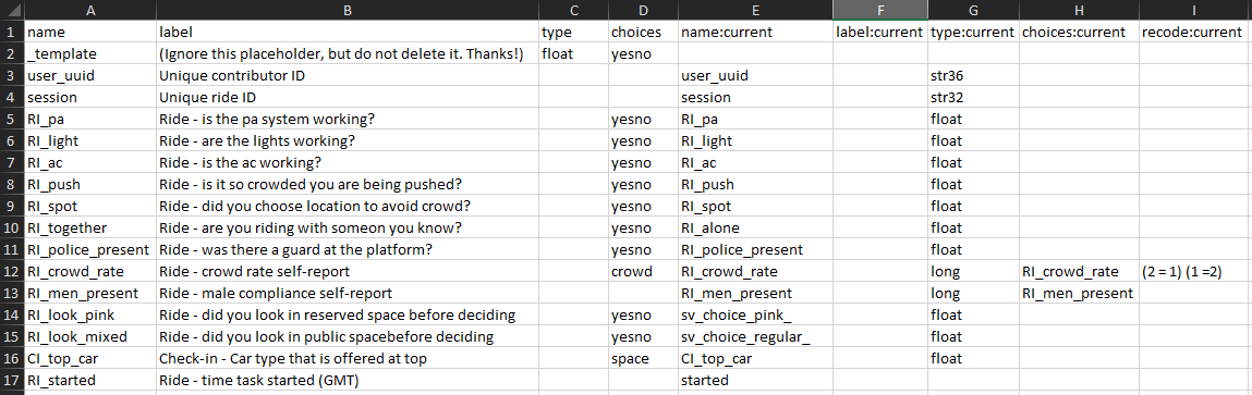
Column B contains the corrected variable labels, column D indicates the value labels to be used for categorical variables, and column I recodes the underlying numbers in those variables. The differences between columns E and A indicate changes to variable names. Typically, it is strongly recommended not to rename variables at the cleaning stage, because it is important to maintain correspondence with the original data set. However, that was not possible in this case, because the same question had inconsistent variable names across multiple transfers of the data from the technology firm managing the mobile application. In fact, this is one of the two cleaning tasks that could not be performed directly through iecodebook (the other was transforming string variables to a categorical format for increased efficiency). The following code shows a few examples of how these cleaning tasks were carried out directly in the script:

    * Encode crowd rate
    encode  ride_crowd_rate, gen(RI_crowd_rate)

    * Reconcile different names for compliance variable
    replace ride_men_present = approx_percent_men if missing(ride_men_present)

    * Encode compliance variable
    encode  ride_men_present, gen(RI_men_present)

    * Did you look in the cars before you made your choice?
    * Turn into dummy from string
    foreach var in sv_choice_pink sv_choice_regular {
        gen `var'_ = (`var' == "Sim") if (!missing(`var') & `var' != "NA")
    }

To document the contents of the original data, the team published supplemental materials on GitHub, including the description of tasks shown in the app. All of the codebooks and Excel sheets used by the code to clean and correct data were also included in the documentation folder of the reproducibility package.

For the complete do-file for cleaning the ride task, visit the GitHub repository at https://git.io/Jtgqj. For the corresponding codebook, visit the GitHub repository at https://git.io/JtgNS.

Documenting data cleaning

Throughout the data-cleaning process, extensive inputs are often needed from the people responsible for data collection. Sometimes this is the research team, but often it is someone else. For example, it could be a survey team, a government ministry responsible for administrative data systems (for an example, see Fernandes, Hillberry, and Alcántara (2015)), or a technology firm that generates remote-sensing data. Regardless of who originally collected the data, it is necessary to acquire and organize all documentation describing how the data were generated. The type of documentation¹⁰⁰ available depends on how the data were collected. For original data collection, it should include field protocols, data collection manuals, survey instruments, supervisor notes, and data quality monitoring reports. For secondary data, the same type of information is useful but often not available unless the data source is a well-managed data publication. Independent of its exact composition, the data documentation should be stored alongside the data dictionary and codebooks. These files will probably be needed during analysis, and they should be published along with the data, so other researchers may use them for their analysis as well.

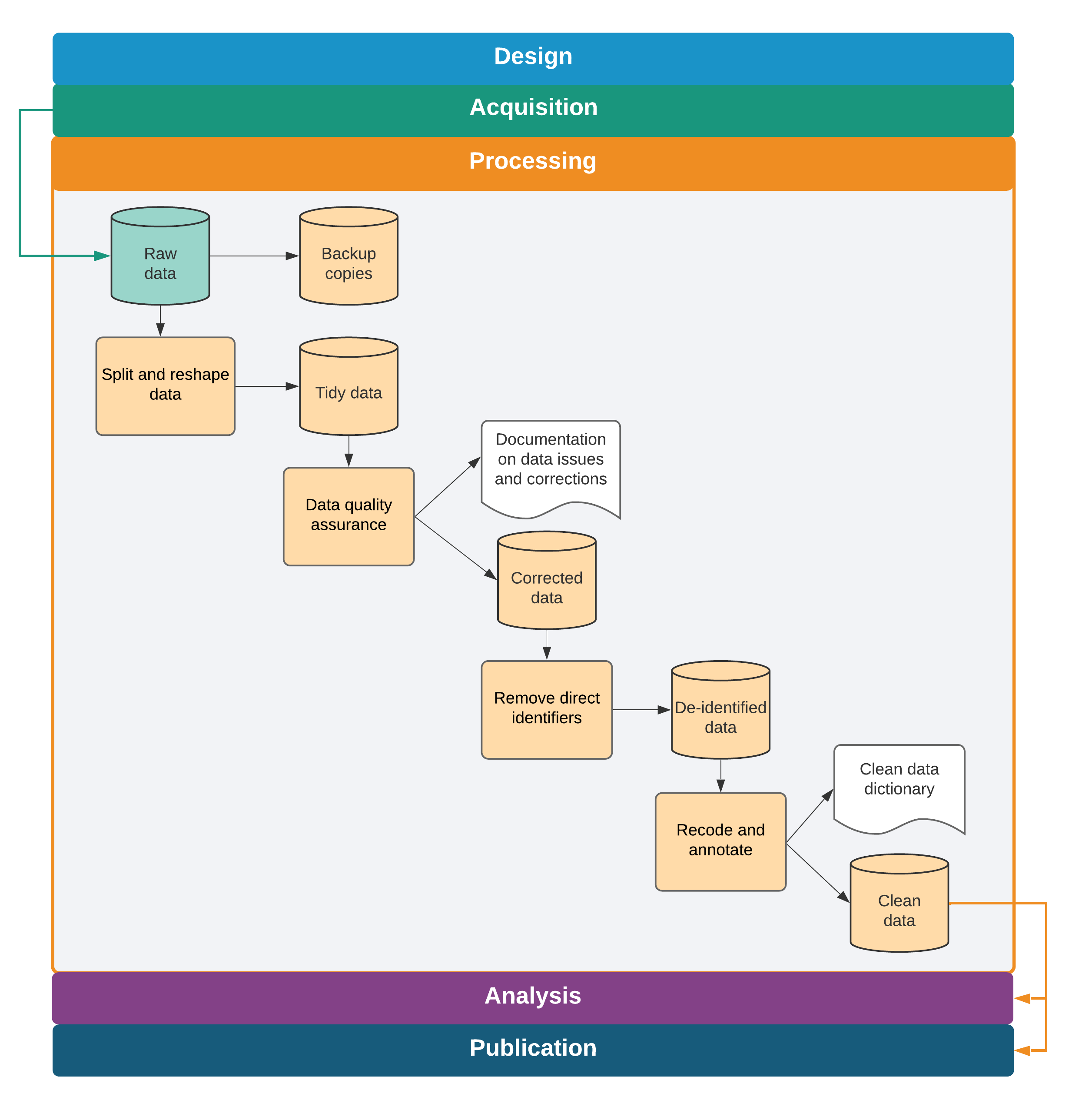
FIGURE 5.1 Data-cleaning tasks and outputs

Source: DIME (Development Impact Evaluation), World Bank.

Looking ahead

This chapter introduced a workflow for formatting, cleaning, and assuring the quality of original data acquired from the field or from partners, illustrated in figure 5.1. These tasks create the first research output when using original data: a clean data set. This data set is well structured to describe the units of analysis (it is “tidy”), it faithfully represents the measurements it was intended to collect, and it does not expose the identities of the people described by it. The team has taken the time to understand the patterns and structures in the data and has annotated and labeled them for use by the team and by others. Combined with the data map, this data set is the fundamental starting point for all analysis work. Chapter 6 describes the steps needed to run the analyses originally specified in the analysis plan and answer the research question—or perhaps to generate even more questions.

Data tables are data that are structured into rows and columns. They are also called tabular data sets or rectangular data. By contrast, nonrectangular data types include written text, NoSQL files, social graph databases, and files such as images or documents.↩︎
The unit of observation is the type of entity that is described by a given data set. In tidy data sets, each row should represent a distinct entity of that type. For more details, see the DIME Wiki at https://dimewiki.worldbank.org/Unit_of_Observation.↩︎
A unique identifier is a variable or combination of variables that distinguishes each entity described in a data set at that level of observation (for example, person, household) with a distinct value. For more details, see the DIME Wiki at https://dimewiki.worldbank.org/ID_Variable_Properties.↩︎
The data linkage table is the component of a data map that lists all the data sets in a particular project and explains how they are linked to each other. For more details and an example, see the DIME Wiki at https://dimewiki.worldbank.org/Data_Linkage_Table.↩︎
A master data set is the component of a data map that lists all individual units for a given level of observation in a project. For more details and an example, see the DIME Wiki at https://dimewiki.worldbank.org/Master_Data_Set.↩︎
A project identifier (ID) is a research design variable used consistently throughout a project to identify observations. For each level of observation, the corresponding project ID variable must uniquely and fully identify all observations in the project. For more details, see the DIME Wiki at https://dimewiki.worldbank.org/ID_Variable_Properties.↩︎
ieduplicates is a Stata command to identify duplicate values in ID variables. It is part of the iefieldkit package. For more details, see the DIME Wiki at https://dimewiki.worldbank.org/ieduplicates.↩︎
iecompdup is a Stata command to compare duplicate entries and understand why they were created. It is part of the iefieldkit package. For more details, see the DIME Wiki at https://dimewiki.worldbank.org/iecompdup.↩︎
A variable is the collection of all data points that measure the same attribute for each observation.↩︎
An observation is the collection of all data points that measure attributes for the same instance of the unit of observation in the data table.↩︎
Wide format refers to a data table in which the data points for a single variable are stored in multiple columns, one for each subunit. In contrast, long format refers to a data table in which a subunit is represented in one row and values representing its parent unit are repeated for each subunit.↩︎
Reshape means to transform a data table in such a way that the unit of observation it represents changes.↩︎
Data quality assurance checks or simply data quality checks are the set of processes put in place to detect incorrect data points due to survey programming errors, data entry mistakes, misrepresentation, and other issues. For more details, see the DIME Wiki at https://dimewiki.worldbank.org/Monitoring_Data_Quality.↩︎
High-frequency data quality checks (HFCs) are data quality checks run in real time during data collection so that any issues can be addressed while the data collection is still ongoing. For more details, see the DIME Wiki at https://dimewiki.worldbank.org/High_Frequency_Checks.↩︎
Duplicate observations are instances in which two or more rows of data are identified by the same value of the ID variable or in which two or more rows unintentionally represent the same respondent. They can be created by situations such as data entry mistakes in the ID variable or repeated surveys or submissions. For more details, see the DIME Wiki at https://dimewiki.worldbank.org/Duplicates_and_Survey_Logs.↩︎
Personally identifying information (PII) is is any piece or set of information that can be linked to the identity of a specific individual. For more details, see the DIME Wiki at https://dimewiki.worldbank.org/Personally_Identifiable_Information_(PII) and pillar 4 of the DIME Research Standards at https://github.com/worldbank/dime-standards.↩︎
Human subjects are any living individuals about whom a research team collects data through intervention or interaction with them, as well as any living individuals who can be identified readily using research data. For more details, see the DIME Wiki at https://dimewiki.worldbank.org/Protecting_Human_Research_Subjects.↩︎
De-identification is the process of removing or masking PII to reduce the risk that subjects’ identities can be connected with the data. For more details, see the DIME Wiki at https://dimewiki.worldbank.org/De-identification. ↩︎
iecodebook is a Stata command to document and execute repetitive data-cleaning tasks such as renaming, recoding, and labeling variables; to create complete codebooks for data sets; and to harmonize and append data sets containing similar variables. It is part of the iefieldkit package. For more details, see the DIME Wiki at https://dimewiki.worldbank.org/iecodebook. ↩︎
Data construction is the process of developing analysis data sets from information or data obtained as part of research, including variable creation, changes in unit of analysis, data integration, and data subsetting.↩︎
In statistical software, categorical variables are stored as numeric integers, each representing one category. Value labels or levels are the names assigned to each category in a categorical variable in Stata and R, respectively. For more details, see the DIME Wiki at https://dimewiki.worldbank.org/Data_Cleaning.↩︎
Survey codes are values that are used as placeholders in survey questions to indicate types of outcomes other than responses to the question, such as refusal to answer. For more details, see the DIME Wiki at https://dimewiki.worldbank.org/Data_Cleaning.↩︎
Variable labels are short descriptors of the information contained in a variable in statistical software. For more details, see the DIME Wiki at https://dimewiki.worldbank.org/Data_Cleaning.↩︎
Data documentation is the process of systematically recording information related to research data work. For more details, see the DIME Wiki at https://dimewiki.worldbank.org/Data_Documentation.↩︎