Chapter 3 Establishing a measurement framework
The first step in the data workflow is to establish a measurement framework, which requires understanding a project’s data requirements and how to structure the required data to answer the research questions. Setting up the measurement framework involves more than simply listing the key outcome variables. It is also necessary to understand how to structure original data, to determine how different data sources connect together, and to create tools to document these decisions and communicate them to the full research team. This chapter shows how to develop this framework and demonstrates that planning in advance saves time and improves the quality of research.
The first section of this chapter introduces the DIME data map template. The template includes a data linkage table, master data sets, and data flowcharts. These tools are used to communicate the project’s data requirements across the team and over time. The second section describes how to translate a project’s research design into data needs. It provides examples of the specific data required by common types of impact evaluation research designs and how to document the link between research design and data sources in the data map template. The final section links the measurement framework to the reproducibility and credibility pillars introduced in chapter 1. It covers how to generate research design variables that are reproducible and how to use power calculations and randomization inference to assess credibility. Box 3.1 summarizes the most important points, lists the responsibilities of different members of the research team, and provides a list of key tools and resources for implementing the recommended practices.
BOX 3.1 SUMMARY: ESTABLISHING A MEASUREMENT FRAMEWORK
To be useful for research, original data must be mapped to a research design through a measurement framework. The measurement framework links each of the project’s data sets to the research design and establishes their connections and relationships. Elaborating the measurement framework at the start of a research project ensures that all team members have the same understanding and creates documentation that will prove useful over the full research cycle. The measurement framework includes three key outputs.
- Data map. The data map documents all of the data for the project. The materials in the data map provide documentation for
- All data sets, units of observation, and high-level relationships between data sets, which are provided in a data linkage table;
- The master data sets for each unit of observation, which define the statistical populations of interest; and
- The expected ways in which data sets will be combined in data processing and analysis, with data flowcharts as a visual guide.
- Research design variables. The research design variables, which translate the research design into data, describe characteristics like the following:
- Treatment and sampling variables, such as comparison groups, clusters and strata, and other variables, which describe how units of observation relate to the proposed analytical methodology
- Time variables, which may be regular or irregular and serve to structure the data temporally
- Monitoring indicators, which characterize the implementation of interventions or surveys
- Outputs of random processes. Random processes, implemented through statistical software, are often needed to translate research designs into data work. These random processes share common characteristics and can include the following:
- Random sampling, to choose a subset of the population of interest to observe
- Random treatment assignment, to determine which units will be placed into which experimental condition in a randomized trial
- More complex designs, such as clustering or stratification, which require special considerations
Key responsibilities for task team leaders and principal investigators
- Oversee and provide inputs to the development of data linkage tables, master data set(s), and data flowchart(s); and review and approve the complete data map.
- Supervise the generation of all research design variables required to execute the study design, and establish guidelines for any research design variables that require data collection.
- Provide detailed guidance on the expected function and structure of random processes.
Key responsibilities for research assistants
- Develop all components of the data map template, and maintain them throughout the project life cycle, documenting any changes to the structure of data or units of observation.
- Understand the study design and how it translates to the project’s data structure.
- Generate all research design variables transparently and reproducibly, taking care to follow the best-practice protocols for random processes.
Key Resources
The following detailed articles on the DIME Wiki website explain the components of the data map:
- Data linkage table at https://dimewiki.worldbank.org/Data_Linkage_Table
- Master data sets at https://dimewiki.worldbank.org/Master_Data_Set
- Data flowchart at https://dimewiki.worldbank.org/Data_Flow_Charts
Appendix C of this book includes intuitive descriptions of common impact evaluation research designs, targeted to research staff without doctoral-level training, such as research assistants and field coordinators.
Documenting data needs
Most projects require more than one data source to answer a research question. Data could be sourced from multiple survey rounds, acquired from various partners (such as administrative data or implementation data), acquired from technological tools like satellite imagery or web scraping, or sourced from complex combinations of these and other sources (for an example, see Kondylis and Stein (2018)). Regardless of how the study data are structured, it is essential to know how to link data from all sources and analyze the relationships between units to answer the research questions. It is not possible to keep all of the relevant details straight without a structured process because the whole research team is unlikely to have the same understanding, over the whole life cycle of the project, of the relationship between all of the required data sets. To ensure that the full team shares the same understanding, best practice is to create a data map32. The data map is intended to ensure that all of the data are in hand to answer the intended research questions, well before starting the analysis described in chapter 6. The data map provides documentation for the project. The process of drafting the data map provides a useful opportunity for principal investigators to communicate their vision of the data structure and requirements and for research assistants to communicate their understanding of that vision. The recommended best practice is to complete the data map before acquiring any data and to make it part of the preregistration of the study. However, in practice many research projects evolve as new data sources, observations, and research questions arise, which means that each component of the data map has to be maintained and updated continuously.
The DIME data map template has three components: one data linkage table, one or several master data sets, and one or several data flowcharts. The data linkage table33 lists all of the original data sets that will be used in the project, what data sources they are created from, and how they relate to each other. For each unit of observation in the data linkage table as well as for each unit of analysis to be used, a master data set34 is created and maintained, listing all observations of the unit that are relevant to the project. Finally, using these two resources, data flowcharts35 are created, describing how the original data sets and master data sets are to be combined and transformed to create analysis data sets. Each component is discussed in more detail in the following subsections.
In order to map measurement frameworks into data needs, it is helpful to distinguish between two types of variables: variables that tie the research design to observations in the data, which are called research design variables, and variables that correspond to observations of the real world, which are called measurement variables. Research design variables map information about the research subjects onto the research design. Often, these variables have no meaning outside of the research project—for example, identification variables and treatment status. Others are observations from the real world, but only those that determine how each specific research unit should be handled during the analysis—for example, treatment uptake and eligibility status. Measurement variables, in contrast, are real-world measures that are not determined by the research team. Examples include characteristics of the research subject, outcomes of interest, and control variables, among many others.
Developing a data linkage table
To create a data map according to the DIME template, the first step is to create
a data linkage table by listing in a spreadsheet all of the data sources that
will be used and the original data sets that will be created from them. If one
source of data will result in two different data sets, then each data set is
listed on its own row. For each data set, the unit of observation and the name
of the project identifier36 (ID)
variable for that unit of observation are listed. It is important to include
both plain-language terminology as well as technical file and variable names
here. For example, the hh_baseline2020_listmap.csv data set may be titled the
“Baseline Household Listing” data; it may be identified by the hh_id
variable and listed as being identified at the household level. Establishing
such plain-language terminology early in the project allows the team to use
these labels unambiguously in communication.
The data linkage table is useful for planning how each unit of observation will be identified in the data. When a data set is listed in the data linkage table, which should be done before the data set is acquired, it is important to ensure that the data will be fully and uniquely identified by the project ID or to plan how the new data set will be linked to the project ID. Working with a data set that does not have an unambiguous link to the project ID is very labor-intensive and a major source of error (for an example of credible matching across data sets in the absence of a unique ID, see Fernandes, Hillberry, and Mendoza Alcantara (2017)).
When combining data sets, the data linkage table should indicate whether data sets can be merged one-to-one or appended (for example, with baseline and endline data sets that use the same unit of observation) or whether two data sets need to be merged many-to-one (for example, merging school administrative data with student data). The data map must indicate which ID variables can be used—and how—when combining data sets. The data linkage table is also a great place to list other metadata, such as the source of the data, its backup locations, the nature of the data license, and so on (see the example in box 3.2).
BOX 3.2 DEVELOPING A DATA LINKAGE TABLE: AN EXAMPLE FROM THE DEMAND FOR SAFE SPACES PROJECT
The main unit of observation in the platform survey data sets was the
respondent, uniquely identified by the variable ID. However, implicit
association tests (IATs) were collected through a specialized software that
produced output from two data sets for each IAT instrument: one at the
respondent level, containing the final scores, and one with detailed information
on each stimulus used in the test (images or expressions to be associated with
concepts). Three IAT instruments were used: one testing the association between
gender and career choice, one testing the association between car choice and
safety concerns, and one testing the association between car choice and openness
to sexual advances.
As a result, the original data for the platform survey component of the project consisted of seven data sets: one for the platform survey and six for the IAT—three with IAT scores (one for each instrument) and three with detailed stimuli data (one for each instrument). All seven data sets were stored in the same raw data folder. The data linkage table listed their filenames and indicated how their ID variables are connected. In the table below, the raw stimulus data do not have a unique identifier, because the same stimulus can be shown repeatedly, so the “ID var” field is blank for these data sets.
| Data source | Raw dataset name | Unit of observation (ID var) |
Parent unit (ID var) |
|---|---|---|---|
| Platform survey | platform_survey_raw_deidentified.dta | respondent (id) | |
| Gender-career implicit association test | career_stimuli.dta | stimulus | respondent (id) question block (block) |
| Car choice-safety concerns implicit association test | security_stimuli.dta | stimulus | respondent (id) question block (block) |
| Car choice-openness to advances implicit association test | reputation_stimuli.dta | stimulus | respondent (id) question block (block) |
| Gender-career implicit association test | career_score.dta | respondent (id) | |
| Car choice-safety concerns implicit association test | security_score.dta | respondent (id) | |
| Car choice-openness to advances implicit association test | reputation_score.dta | respondent (id) |
The complete project data map is available at https://git.io/Jtg3J.
Constructing master data sets
The second step in creating a data map is to create one master data set for each unit of observation that will be used in any research activity. Examples of such activities are data collection, data analysis, sampling, and treatment assignment. The master data set is the authoritative source of the project ID and all research design variables for the corresponding unit of observation, such as sample status and treatment assignment. Therefore, the master data set serves as an unambiguous method of mapping the observations in the data to the research design. A master data set should not include any measurement variables. Research design variables and measurement variables may come from the same source, but should not be stored in the same way. For example, if the project acquires administrative data that include both information on eligibility for the study (research design variables) and data on the topic of study (measurement variables), the research design variables should be stored in the master data set, and the measurement variables should be stored separately and prepared for analysis as described in chapter 5.
Each master data set is to be the authoritative source for how all observations at that unit of analysis are identified. Therefore, the master data sets should include identifying information such as names, contact information, and project ID. The project ID is the ID variable used in the data linkage table and is therefore used to link observations across data sets. The master data set may list alternative IDs—for example, IDs used by a partner organization—but an alternative ID should never be used as the project ID, because doing so would allow individuals outside the research team to identify the research subjects. The project team must create the project ID, and the linkage to direct identifiers should be accessible only to people listed on the protocol approved by the institutional review board. The master data set serves as the link between all other identifying information and the project ID. Because the master data set is full of directly identifying information, it must always be encrypted. If a data set is received with an alternative ID, it should be replaced with the project ID as a part of the de-identification process (see chapters 5 and 7 for more on de-identification). The alternative ID should be stored in the master data set so that it may be linked back to the data using the project ID if needed. Any data set that needs to retain an alternative ID for any reason should be treated as confidential data; it should always be encrypted and never published.
The starting point for the master data set is typically a sampling frame (more on sampling frames later in this chapter). However, it is essential to update the master data set continuously with all observations encountered in the project, even if those observations are not eligible for the study. Examples include new observations that are listed during monitoring activities or observations that are connected to respondents in the study—for example, in a social network module. This updating is useful because errors become less likely in record linkages such as fuzzy matching using string variables as more information is added to the master data set. If it is ever necessary to perform a fuzzy match to a data source that does not have a unique ID, this task should be done using the master data set (for an example, see Benhassine et al. (2018)). Data from sources that are not fully and uniquely identified with the project ID should not be cleaned or analyzed until the project IDs have been merged successfully from the master data set. If this process results in the project adding new observations to the master data set, it is necessary to confirm beyond a reasonable doubt that the new observation is indeed a new observation and not simply a failed match to an observation already contained in the master data set. For example, it should be checked whether identifiers such as proper names have inconsistent spellings or romanizations or whether identifiers such as addresses or phone numbers have become outdated.
Creating data flowcharts
The third and final step in creating the data map is to create data flowcharts. Each analysis data set (see chapter 6 for a discussion on why multiple analysis data sets may be needed) should have a data flowchart showing how it was created. The flowchart is a diagram in which each starting point is either a master data set or a data set listed in the data linkage table. The data flowchart should include instructions on how the original data sets can be combined to create the analysis data set. The operations used to combine the data could include appending, one-to-one merging, many-to-one or one-to-many merging, collapsing, reshaping, or a broad variety of other operations. It is important to list which variable or set of variables should be used in each operation and to note whether the operation creates a new variable or a combination of variables to identify the newly linked data. Data sets should be linked by project IDs when possible (exceptions are time variables in longitudinal data and subunits like farm plots, which correspond to a farmer with a project ID but do not themselves have project IDs). Once the data sets listed in the flowchart have been acquired, the number of observations that the starting point data set has and the number of observations that each resulting data set should have after each operation can be added to the data flowcharts. This method is useful for tracking attrition and making sure that the operations used to combine data sets do not create unwanted duplicates or incorrectly drop any observations.
The information that goes into the data flowcharts can be expressed in text, but diagrams generally are the most efficient way to communicate this information across a team (see the example in box 3.3). A data flowchart can be created using a flowchart drawing tool (many free options are available online) or using the shapes or tools in Microsoft Office. It can also be created simply by drawing on a piece of paper and taking a photo, but a digital tool is recommended so that flowcharts can be updated easily over time if needed. As with the data linkage table, the flowchart should include both technical information and plain-language interpretations of the operations that are done and the data that are created. This information is useful for understanding the complex data combinations that often result from merges and appends, such as panel data sets like “person-year” structures and multilevel data like “district-school-teacher-student” structures.
The flowchart summarizes each operation that changes the level of observation of the data and how data sets will be combined. Because these changes are the most error-prone data-processing tasks, having a high-level plan for how they will be executed helps to clarify the process for everyone on the data team, preventing future mistakes.
BOX 3.3 CREATING DATA FLOWCHARTS: AN EXAMPLE FROM THE DEMAND FOR SAFE SPACES PROJECT
The data flowchart indicates how the original data sets were processed and
combined to create a final respondent-level data set that was used for analysis.
In figure B3.3.1, the analysis data set resulting from this process is shown in
green. The original data sets are shown in blue (refer to the sample in box 3.2
for details on the original data sets). The name of the uniquely identifying
variable in the data set is indicated in the format (ID: variable_name).
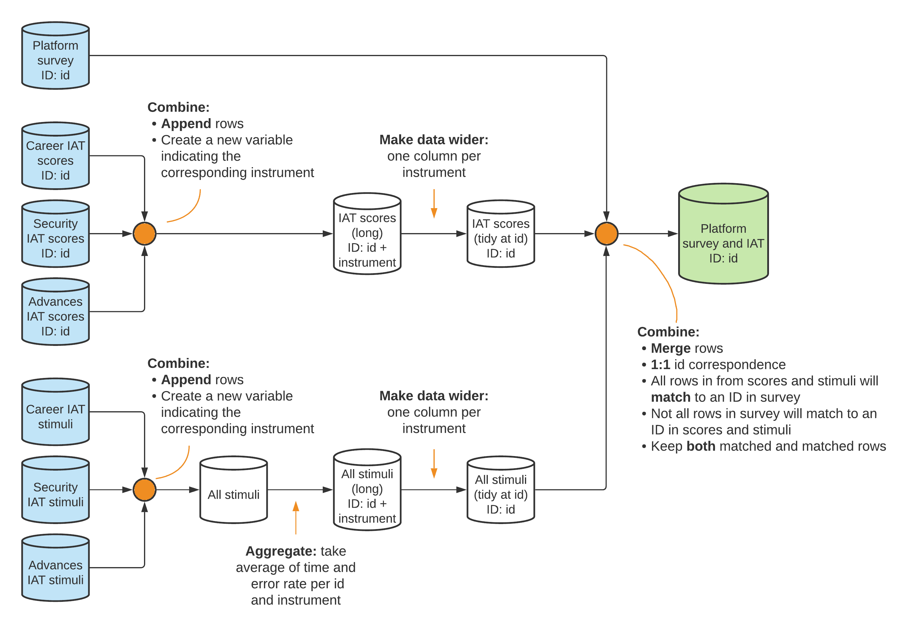
Source: For the complete project data map, visit the GitHub repository at
https://git.io/Jtg3J
Note: IAT = implicit association test; ID = identifying
variable.
Translating research design to data needs
An important step in translating the research design into a specific data structure is to determine which research design variables are needed to infer which differences in measurement variables are attributable to the research design. These data needs should be expressed in the data map by listing the data source for each variable in the data linkage table, by adding columns for them in the master data set (the master data set might not have any observations yet; that is not a problem), and by indicating in the data flowcharts how they will be merged with the analysis data. It is important to perform this task before acquiring any data, to make sure that the data acquisition activities described in chapter 4 will generate the data needed to answer the research questions.
Because DIME works primarily on impact evaluations, the discussion here focuses on research designs that compare a group that received some kind of treatment37 against a counterfactual38. The key assumption is that each person, facility, or village (or whatever the unit of analysis is) has two possible states: the outcome if the unit did receive the treatment and the outcome if it did not receive the treatment. The average treatment effect39 (ATE) is the difference between these two states averaged over all units.
However, it is impossible to observe the same unit in both the treated and
untreated state simultaneously, so it is impossible to calculate these
differences directly. Instead, the treatment group is compared to a control
group that is statistically indistinguishable, which is often referred to as
achieving balance between two or more groups. DIME Analytics maintains a Stata
command to standardize and automate the creation of well-formatted balance
tables: iebaltab (for instructions and details, see the DIME Wiki at
https://dimewiki.worldbank.org/iebaltab). Each research design has a different
method for identifying and balancing the counterfactual group. The rest of this
section covers how different methods require different research data. What does
not differ, however, is that these data requirements are all research design
variables that should always be included in the master data set. It is usually
necessary to merge the research design variables with other data sets many times
during a project, but this task is easy if the project has created a data
linkage table.
This chapter assumes that the reader has a working familiarity with the research designs mentioned here. Appendix C provides more details and specific references for common types of impact evaluation designs.
Applying common research designs to data
When using experimental methods40, such as randomized control trials41 (RCTs), the research team determines which members of the studied population will receive the treatment. This decision is typically made by a randomized process in which a subset of the eligible population is randomly assigned to receive the treatment (implementation is discussed later in this chapter). The intuition is that, if everyone in the eligible population is assigned at random to either the treatment or the control group, the two groups will, on average, be statistically indistinguishable. Randomization makes it generally possible to obtain unbiased estimates of the effects that can be attributed to a specific program or intervention: in a randomized trial, the expected spurious correlation between treatment and outcomes will approach zero as the sample size increases (Duflo, Glennerster, and Kremer (2007), Gibson and Sautmann (2020)). The randomized assignment should be done using data from the master data set, and the result should be saved back to the master data set before being merged with other data sets.
Quasi-experimental methods42, by contrast, are based on events not controlled by the research team. Instead, they rely on “experiments of nature,” in which natural variation in exposure to treatment can be argued to approximate deliberate randomization. This natural variation has to be measured, and the master data set has to document how the variation is categorized as outcomes of a naturally randomized assignment. Unlike carefully planned experimental designs, quasi-experimental designs typically require the luck of having access to data collected at the right times and places to exploit events that occurred in the past. Therefore, these methods often use either secondary data, including administrative data, or other classes of routinely collected information; and it is important for the data linkage table to document how these data can be linked to the rest of the data in the project.
Regardless of the type of design, it is necessary to be very clear about which of the data points observed or collected are research design variables. For example, regression discontinuity43 (RD) designs exploit sharp breaks or limits in policy designs (for an example, see Alix-Garcia et al. (2019)). The cutoff determinant—or running variable—should be saved in the master data set. In instrumental variables44 (IV) designs, the instruments influence the probability of treatment (for an example, see Calderon, Iacovone, and Juarez (2017)). These research design variables should be collected and stored in the master data set. Both the running variable in RD designs and the instruments in IV designs are among the rare examples of research design variables that may vary over time. In such cases, the research design should clearly indicate ex ante the point in time when they will be recorded, and this information should be clearly documented in the master data set.
In matching45 designs, statistically similar observations are identified using strata, indexes, or propensity scores unrelated to the topic of the study. Matching can be used to pair units that already have or will receive the treatment to identify statistically similarly control units. It can also be used to identify pairs or groups of statistically similar units within which the research team randomizes who will be treated. Like all research design variables, the matching results should be stored in the master data set. This recording is best done by assigning a matching ID to each group and creating a variable in the master data set with the matching ID to which each unit belongs (for an example, see Prennushi and Gupta (2014)).
Including multiple time periods
The data map should also consider whether the project uses data from one time period or several. A study that observes data in only one time period is called a cross-sectional study. Observations over multiple time periods, referred to as longitudinal data, can consist of either repeated cross sections or panel data. In repeated cross sections, each successive round of data collection uses a new sample of units from the treatment and control groups (which may or may not overlap), whereas in a panel data study the same units are tracked and observed in each round (for an example, see Kondylis et al. (2016)). If each round of data collection is a separate activity, then each round should be treated as a separate source of data and given its own row in the data linkage table.
Data that are generated continuously or are acquired at frequent intervals can be treated as a single data source. When data are acquired in discrete batches, the data linkage table must document how the different rounds will be combined. It is important to keep track of the attrition rate in panel data, which is the share of intended observations not observed in each round of data collection. The characteristics of units that are not possible to track are often correlated with the outcome being studied (for an example, see Bertrand et al. (2017)). For example, poorer households may live in more informal dwellings, patients with worse health conditions might not survive to follow-up, and so on. If this is the case, then estimated treatment effects might in reality only be an artifact of the remaining sample being a subset of the original sample that were better or worse off from the beginning. A research design variable in the master data set is needed to indicate attrition. A balance check using that attrition variable can provide insights about whether the lost observations are systematically different from the rest of the sample.
Incorporating monitoring data
For any study with an ex ante design, monitoring data46 are very important for understanding whether the research design corresponds to reality. The most typical example is to make sure that, in an experimental design, the treatment is implemented according to the treatment assignment. Treatment is often implemented by partners, and field realities may be more complex than foreseen during research design. Furthermore, field staff of the partner organization might not be aware that they are implementing a research design.
In all impact evaluation research designs, fidelity to the design is important to record as well (for an example, see Pradhan et al. (2013)). For example, a program intended for students who scored under 50 percent on a test might have some cases in which the program was offered to someone who scored 51 percent on the test and participated in the program or someone who scored 49 percent on the test but declined to participate in the program. Differences between assignments and realizations should also be recorded in the master data sets. Therefore, for nearly all research designs, it is essential to acquire monitoring data to indicate how well the realized treatment implementation in the field corresponds to the intended treatment assignment.
Although monitoring data have traditionally been collected by someone in the field, it is increasingly common for monitoring data to be collected remotely. Some examples of remote monitoring include the use of local collaborators to upload geotagged images for visible interventions (such as physical infrastructure), the installation of sensors to broadcast measurements (such as air pollution or water flow), the distribution of wearable devices to track location or physical activity, or the application of image recognition to satellite data. In-person monitoring activities are often preferred, but cost and travel dangers, such as conflicts or disease outbreaks, make remote monitoring innovations increasingly appealing. If cost alone is the constraint, it is worthwhile to consider monitoring a subset of the implementation area in person. The information collected may not be detailed enough to be used as a control in the analysis, but it will provide a means to estimate the validity of the research design assumptions.
Linking monitoring data to the rest of data in the project is often complex and a major source of errors. Monitoring data are rarely received in the same format or structure as research data (for an example, see Goldstein et al. (2015)). For example, the project may receive a list of the names of all people who attended a training or administrative data from a partner organization without any unique ID. In both of these cases, it can be difficult to ensure a one-to-one match between units in the monitoring data and the master data sets. Planning ahead and collaborating closely with the implementing organization from the outset of the project are the best ways to avoid these difficulties. Often, it is ideal for the research team to prepare forms (paper or electronic) for monitoring, preloading them with the names of sampled individuals or ensuring that a consistent ID is directly linkable to the project ID. If monitoring data are not handled carefully and actively used in fieldwork, treatment implementation may end up being poorly correlated with treatment assignment, without a way to tell if the lack of correlation is a result of bad matching of monitoring data or a meaningful problem of implementation.
Creating research design variables by randomization
Random sampling and random treatment assignment are two core research activities that generate important research design variables. These processes directly determine the set of units that will be observed and what their status will be for the purpose of estimating treatment effects. Randomization47 is used to ensure that samples are representative and that treatment groups are statistically indistinguishable. Randomization is often used to produce random samples and random treatment assignments. In this book, the term “randomization” is used only to describe the process of generating a sequence of unrelated numbers, even though it is often used in practice to refer to random treatment assignment.
Randomization in statistical software is nontrivial, and its mechanics are not intuitive for the human mind. The principles of randomization apply not just to random sampling and random assignment but also to all statistical computing processes that have random components, such as simulations and bootstrapping. Furthermore, all random processes introduce statistical noise or uncertainty into the estimates of effect sizes. Choosing one random sample from all of the possibilities produces some probability of choosing a group of units that are not, in fact, representative. Similarly, choosing one random assignment produces some probability of creating groups that are not good counterfactuals for each other. Power calculation and randomization inference are the main methods by which these probabilities of error are assessed. These analyses are particularly important in the initial phases of development research—typically conducted before any data acquisition or field work occur—and have implications for feasibility, planning, and budgeting.
Randomizing sampling and treatment assignment
Random sampling is the process of randomly selecting observations from a list of units to create a subsample that is representative or that has specific statistical properties (such as selecting only from eligible units, oversampling populations of interest, or other techniques such as weighted probabilities). This process can be used, for example, to select a subset from all eligible units to be included in data collection when the cost of collecting data on everyone is prohibitive. For more details on sampling, see the DIME Wiki at https://dimewiki.worldbank.org/Sampling. It can also be used to select a subsample of observations to test a computationally heavy process before running it on the full data.
Randomized treatment assignment is the process of assigning observations to different treatment arms. This process is central to experimental research design. Most of the code processes used for randomized assignment are the same as those used for sampling, which also entails randomly splitting a list of observations into groups. Whereas sampling determines whether a particular unit will be observed at all in the course of data collection, randomized assignment determines whether each unit will be observed in a treatment state or in a counterfactual state.
The list of units to sample or assign from may be called a sampling universe, a listing frame, or something similar. In almost all cases, the starting point for randomized sampling or assignment should be a master data set, and the result of the randomized process should always be saved in the master data set before it is merged with any other data. The only exceptions are when the sampling universe cannot be known in advance. For example, randomized assignment cannot start from a master data set when sampling is done in real time, such as randomly sampling patients as they arrive at a health facility or when treatment is assigned through an in-person lottery. In those cases, it is important to collect enough data during real-time sampling or to prepare the inputs for the lottery such that all units can be added to the master data set afterward.
The simplest form of sampling is uniform-probability random sampling, which means that every eligible observation in the master data set has an equal probability of being selected. The most explicit method of implementing this process is to assign random numbers to all of the potential observations, order them by the number they are assigned, and mark as “sampled” those with the lowest numbers, up to the desired proportion. It is important to become familiar with exactly how the process works. The do-file in box 3.4 provides an example of how to implement uniform-probability sampling in practice. The code there uses a Stata built-in data set and is fully reproducible (more on reproducible randomization in next section), so anyone who runs this code in any version of Stata later than 13.1 (the version set in this code) will get the exact same, but still random, results.
BOX 3.4 AN EXAMPLE OF UNIFORM-PROBABILITY RANDOM SAMPLING
* Set up reproducible randmomization - VERSIONING, SORTING and SEEDING
    ieboilstart, v(13.1)     // Version
    `r(version)'             // Version
    sysuse bpwide.dta, clear // Load data
    isid patient, sort       // Sort
    set seed 215597          // Seed - drawn using https://bit.ly/stata-random

* Generate a random number and use it to sort the observations.
* Then the order the observations are sorted in is random.
    gen  sample_rand = rnormal() // Generate a random number
    sort sample_rand             // Sort based on the random number

* Use the sort order to sample 20% (0.20) of the observations.
* _N in Stata is the number of observations in the active dataset,
* and _n is the row number for each observation. The bpwide.dta has 120
* observations and 120*0.20 = 24, so (_n <= _N * 0.20) is 1 for observations
* with a row number equal to or less than 24, and 0 for all other
* observations. Since the sort order is randomized, this means that we
* have randomly sampled 20% of the observations.
    gen sample = (_n <= _N * 0.20)

* Restore the original sort order
    isid patient, sort

* Check your result
    tab sample
To access this code in do-file format, visit the GitHub repository at https://github.com/worldbank/dime-data-handbook/tree/main/code.
Sampling typically has only two possible outcomes: observed and unobserved. Similarly, a simple randomized assignment has two outcomes: treatment and control; the logic in the code is identical to the sampling code example. However, randomized assignment often involves multiple treatment arms, each representing different varieties of treatment to be delivered (for an example, see De Andrade, Bruhn, and McKenzie (2013)); in some cases, multiple treatment arms are intended to overlap in the same sample. Randomized assignment can quickly grow in complexity, and it is doubly important to understand fully the conceptual process described in the experimental design and to fill in any gaps before implementing it in code. The do-file in box 3.5 provides an example of how to implement randomized assignment with multiple treatment arms.
BOX 3.5 AN EXAMPLE OF RANDOMIZED ASSIGNMENT WITH MULTIPLE TREATMENT ARMS
* Set up reproducible randomization - VERSIONING, SORTING and SEEDING
    ieboilstart, v(13.1)     // Version
    `r(version)'             // Version
    sysuse bpwide.dta, clear // Load data
    isid patient, sort       // Sort
    set seed 654697          // Seed - drawn using https://bit.ly/stata-random

* Generate a random number and use it to sort the observation.
* Then the order the observations are sorted in is random.
    gen treatment_rand = rnormal() // Generate a random number
    sort treatment_rand            // Sort based on the random number

* See simple-sample.do example for an explanation of "(_n <= _N * X)".
* The code below randomly selects one third of the observations into group 0,
* one third into group 1 and one third into group 2.
* Typically 0 represents the control group
* and 1 and 2 represents the two treatment arms
    generate treatment = 0                       // Set all observations to 0 (control)
    replace  treatment = 1 if (_n <= _N * (2/3)) // Set only the first two thirds to 1
    replace  treatment = 2 if (_n <= _N * (1/3)) // Set only the first third to 2

* Restore the original sort order
    isid patient, sort

* Check your result
    tab treatment
To access this code in do-file format, visit the GitHub repository at https://github.com/worldbank/dime-data-handbook/tree/main/code.
Programming reproducible random processes
For statistical programming to be reproducible, it is necessary to be able to reobtain its exact outputs in the future (Orozco et al. (2018)). This section focuses on what is needed to produce truly random results and to ensure that those results can be obtained again. This effort takes a combination of strict rules, solid understanding, and careful programming. The rules are not negotiable (but thankfully are simple). Stata, like most statistical software, uses a pseudo-random number generator48, which, in ordinary research use, produces sequences of numbers that are as good as random. However, for reproducible randomization49, two additional properties are needed: the ability to fix the sequence of numbers generated and the a bility to ensure that the first number is independently randomized. In Stata, reproducible randomization is accomplished through three concepts: versioning, sorting, and seeding. Stata is used in the examples, but the same principles translate to all other programming languages.
Rule 1: Versioning requires using the same version of the software each time the random process is run. If anything is different, the underlying list of pseudo-random numbers may have changed, and it may be impossible to recover the original result. In Stata, the
versioncommand ensures that the list of numbers is fixed. Most important is to use the same version across a project, but, at the time of writing, using Stata version 13.1 is recommended for backward compatibility. The algorithm used to create this list of random numbers was changed after Stata 14, but the improvements are unlikely to matter in practice. Theieboilstart50 command inietoolkitprovides functionality to support this requirement. Usingieboilstartat the beginning of the master do-file51 is recommended. Testing the do-files without running them via the master do-file may produce different results, because Stata’sversionsetting expires after code execution completes.Rule 2: Sorting requires using a fixed order of the actual data on which the random process is run. Because random numbers are assigned to each observation row by row starting from the top row, changing their order will change the result of the process. In Stata, using
isid [id_variable], sortis recommended to guarantee a unique sorting order. This command does two things. First, it tests that all observations have unique values in the sorting variable, because duplicates would cause an ambiguous sort order. If all values are unique, then the command sorts on this variable, guaranteeing a unique sort order. It is a common misconception that thesort, stablecommand may also be used; however, by itself, this command cannot guarantee an unambiguous sort order and therefore is not appropriate for this purpose. Because the exact order must remain unchanged, the underlying data must remain unchanged between runs. If the number of observations is expected to change (for example, to increase during ongoing data collection), randomization will not be reproducible unless the data are split into smaller fixed data sets in which the number of observations does not change. Those smaller data sets can be combined after randomization.Rule 3: Seeding requires manually setting the start point in the list of pseudo-random numbers. A seed is a single number that specifies one of the possible start points. It should be at least six digits long and contain exactly one unique, different, and randomly created seed for each randomization process. To create a seed that satisfies these conditions, see https://bit.ly/stata-random. (This link is a shortcut to a page of the website https://www.random.org where the best practice criteria for a seed are predefined.) In Stata,
set seed [seed]will set the generator to the start point identified by the seed. In R, theset.seedfunction does the same. To be clear: setting a single seed once in the master do-file is not recommended; instead, a new seed should be set in code right before each random process. The most important task is to ensure that each of these seeds is truly random; shortcuts such as the current date or a previously used seed should not be used. Comments in the code should describe how the seed was selected.
How the code was run needs to be confirmed carefully before finalizing it,
because other commands may induce randomness in the data, change the sorting
order, or alter the place of the pseudo-random number generator. The process for
confirming that randomization has worked correctly before finalizing its results
is to save the outputs of the process in a temporary location, rerun the code,
and use the Stata commands cf or datasignature to ensure that nothing has
changed. It is also advisable to let someone else reproduce the randomization
results on another machine to remove any doubt that the results are
reproducible. Once the result of a randomization is used in the field, there is
no way to correct mistakes. The code in box 3.6 provides an example of a fully
reproducible randomization.
BOX 3.6 AN EXAMPLE OF REPRODUCIBLE RANDOMIZATION
* VERSIONING - Set the version
    ieboilstart, v(13.1)
    `r(version)'

* Load the auto dataset (auto.dta is a test dataset included in all Stata installations)
    sysuse auto.dta, clear

* SORTING - sort on the uniquely identifying variable "make"
    isid make, sort

* SEEDING - Seed picked using https://bit.ly/stata-random
    set seed 287608

* Demonstrate stability after VERSIONING, SORTING and SEEDING
    gen check1 = rnormal()  // Create random number
    gen check2 = rnormal()  // Create a second random number without resetting seed

    set seed 287608         // Reset the seed
    gen check3 = rnormal()  // Create a third random number after resetting seed

* Visualize randomization results. See how check1 and check3 are identical,
* but check2 is random relative to check1 and check3
    graph matrix check1 check2 check3, half
To access this code in do-file format, visit the GitHub repository at https://github.com/worldbank/dime-data-handbook/tree/main/code.
As discussed previously, at times it may not be possible to use a master data set for randomized sampling or treatment assignment (for example, when sampling patients on arrival or through live lotteries). Methods like a real-time lottery typically do not leave a record of the randomization and, as such, are never reproducible. However, a reproducible randomization can be run in advance even without an advance list of eligible units. For example, to select a subsample of patients randomly as they arrive at various health facilities, it is possible to compile a pregenerated list with a random order of “in sample” and “not in sample.” Field staff would then go through this list in order and cross off one randomized result as it is used for a patient.
This method is especially beneficial when implementing a more complex randomization. For example, a hypothetical research design may call for enumerators to undertake the following:
- Sample 10 percent of people observed in a particular location.
- Show a video to 50 percent of the sample.
- Administer a short questionnaire to 80 percent of all persons sampled.
- Administer a longer questionnaire to the remaining 20 percent, with the mix of questionnaires equal between those who were shown the video and those who were not.
In real time, such a complex randomization is much more likely to be implemented correctly if field staff can simply follow a list of the randomized categories for which the project team is in control of the predetermined proportions and the random order. This approach makes it possible to control precisely how these categories are distributed across all of the locations where the research is to be conducted.
Finally, if this real-time implementation of randomization is done using survey software, then the pregenerated list of randomized categories can be preloaded into the questionnaire. Then the field team can follow a list of respondent IDs that are randomized into the appropriate categories, and the survey software can show a video and control which version of the questionnaire is asked. This approach can help to reduce the risk of errors in field randomization.
Implementing clustered or stratified designs
For a variety of reasons, random sampling and random treatment assignment are rarely as straightforward as a uniform-probability draw. The most common variants are clustering and stratification (Athey and Imbens (2017a)). Clustering52 occurs when the unit of analysis is different from the unit of randomization in a research design. For example, a policy may be implemented at the village level or the project may only be able to send enumerators to a limited number of villages, but the outcomes of interest for the study are measured at the household level. In such cases, the higher-level groupings by which lower-level units are randomized are called clusters (for an example, see Keating et al. (2011)).
Stratification53 splits the full set of observations into subgroups, or strata, before performing randomized assignment within each subgroup, or stratum. Stratification ensures that members of each stratum are included in all groups of the randomized assignment process or that members of all groups are observed in the sample. Without stratification, randomization may put all members of a given subgroup into just one of the treatment arms or fail to select any of them into a sample. For both clustering and stratification, implementation is nearly identical in both random sampling and random assignment.
Clustered randomization is procedurally straightforward in Stata, although it typically needs to be performed manually. The process for clustering a sampling or randomized assignment is to randomize on the master data set for the unit of observation of the cluster and then merge the results with the master data set for the unit of analysis. This is a many-to-one merge, and the data map should document how those data sets can be merged correctly. If the project does not yet have a master data set for the unit of observation of the cluster, then it is necessary to create one and update the data map accordingly. When sampling or randomized assignment is conducted using clusters, the cluster ID variable should be clearly identified in the master data set for the unit of analysis because it will need to be used in subsequent statistical analysis. Typically, standard errors for clustered designs must be clustered at the level at which the design is clustered (McKenzie 2017). This clustering accounts for the design covariance within the clusters—the information that, if one unit is observed or treated from that cluster, the other members of the cluster are as well.
Although procedurally straightforward, implementing stratified designs in
statistical software is prone to error. Even for a relatively simple
multiple-arm design, the basic method of randomly ordering the observations will
often create very skewed assignments in the presence of strata (McKenzie 2011).
The user-written randtreat Stata command properly implements stratification
(Carril (2017)). The options and outputs (including messages) from the
command should be reviewed carefully so that it is clear exactly what has been
implemented—randtreat performs a two-step process in which it takes the
straightforward approach as far as possible and then, according to the user’s
instructions, handles the remaining observations in a consistent fashion.
Notably, it is extremely hard to target exact numbers of observations in
stratified designs because exact allocations are rarely round fractions.
Performing power calculations
Random sampling and treatment assignment are noisy processes: it is impossible to predict the result in advance. By design, the exact choice of sample or treatment will not be correlated with the key outcomes, but this lack of correlation is only true “in expectation”—that is, the correlation between randomization and other variables will only be zero on average across a large number of randomizations. In any particular randomization, the correlation between the sampling or randomized assignments and the outcome variable is guaranteed to be nonzero: this is called in-sample or finite-sample correlation.
Because the true correlation (over the “population” of potential samples or assignments) is zero, the observed correlation is considered an error. In sampling, this error is called the sampling error, and it is defined as the difference between a true population parameter and the observed mean due to the chance selection of units. In randomized assignment, this error is called randomization noise and is defined as the difference between a true treatment effect and the estimated effect due to the placement of units in treatment groups. The intuition for both measures is that, from any group, it is possible to find some subsets that have higher-than-average values of some measure and some that have lower-than-average values. The random sample or treatment assignment will fall into one of these categories, and it is necessary to assess the likelihood and magnitude of this occurrence. Power calculation and randomization inference are the two key tools for doing so.
Power calculations report the likelihood that the experimental design will be able to detect the treatment effects of interest given these sources of noise. This measure of power can be described in various ways, each of which has different practical uses. The purpose of power calculations is to identify where the strengths and weaknesses are located and to understand the relative trade-offs that the project will face if the randomization scheme is changed for the final design. It is important to consider take-up rates and attrition when doing power calculations. Incomplete take-up will significantly reduce power, and understanding what minimum level of take-up is required can help to guide field operations (for this reason, monitoring take-up in real time is often critical).
The minimum detectable effect54 (MDE) is the smallest true effect that a given research design can reliably detect. It is useful as a check on whether a study is worthwhile. If, in a field of study, a “large” effect is just a few percentage points or a small fraction of a standard deviation, then it is nonsensical to run a study whose MDE is much larger than that. Given the sample size and variation in the population, the effect needs to be much larger to be statistically detected, so such a study would never be able to say anything about the size of effect that is practically relevant. Conversely, the minimum sample size prespecifies expected effect sizes and indicates how large a study’s sample would need to be to detect that effect, which can determine what resources are needed to implement a useful study.
Randomization inference55 is used to analyze the likelihood that the randomized assignment process, by chance, would have created a false treatment effect as large as the one estimated. Randomization inference is a generalization of placebo tests, because it considers what the estimated results would have been from a randomized assignment that did not happen in reality. Randomization inference is particularly important in quasi-experimental designs and in small samples, in which the number of possible randomizations is itself small. Randomization inference can therefore be used proactively during experimental design to examine the potential spurious treatment effects the exact design is able to produce. If results heap significantly at particular levels or if results seem to depend dramatically on the outcome of randomization for a small number of units, randomization inference will flag those issues before the study is fielded and allow adjustments to the design.
Looking ahead
This chapter introduced the DIME data map template, a toolkit to document a data acquisition plan and to describe how each data source relates to the design of a study. The data map contains research design variables and the instructions for using them in combination with measurement variables, which together form the data set(s) for the analytical work. It then discussed ways to use this planning data to inform and execute research design tasks, such as randomized sampling and assignment, and to produce concrete measures of whether the project design is sufficient to answer the research questions posed. The next chapter turns to data acquisition—the first step toward answering those questions. It details the processes of obtaining original data, whether those data are collected by the project or received from another entity.
A data map is a set of tools to document and communicate the data requirements in a project and how different data can be linked together. For more details, see the DIME Wiki at https://dimewiki.worldbank.org/Data_Map.↩︎
The data linkage table is the component of a data map that lists all the data sets in a particular project and explains how they are linked to each other. For more details and an example, see the DIME Wiki at https://dimewiki.worldbank.org/Data_Linkage_Table.↩︎
A master data set is the component of a data map that lists all individual units for a given level of observation in a project. For more details and an example, see the DIME Wiki at https://dimewiki.worldbank.org/Master_Data_Set.↩︎
A data flowchart is the component of a data map that lists how the data sets acquired for the project are intended to be combined to create the data sets used for analysis. For more details and an example, see the DIME Wiki at https://dimewiki.worldbank.org/Data_Flow_Charts.↩︎
A project identifier (ID) is a research design variable used consistently throughout a project to identify observations. For each level of observation, the corresponding project ID variable must uniquely and fully identify all observations in the project. For more details, see the DIME Wiki at https://dimewiki.worldbank.org/ID_Variable_Properties.↩︎
A treatment is an evaluated intervention or event, which includes things like being offered training or a cash transfer from a program or experiencing a natural disaster, among many others.↩︎
A counterfactual is a statistical description of what would have happened to specific individuals in an alternative scenario—for example, a different treatment assignment outcome.↩︎
An average treatment effect (ATE) is the expected difference in a given outcome between a unit observed in its treated state and the same unit observed in its untreated state for a given treatment.↩︎
Experimental methods are research designs in which the researcher explicitly and intentionally induces variation in an intervention assignment to facilitate causal inference. For more details, see appendix C or the DIME Wiki at https://dimewiki.worldbank.org/Experimental_Methods.↩︎
Randomized control trials (RCTs) are experimental design methods of impact evaluation in which eligible units in a sample are randomly assigned to treatment and control groups. For more details, see the DIME Wiki at https://dimewiki.worldbank.org/Randomized_Control_Trials.↩︎
Quasi-experimental methods are research designs in which the researcher uses natural or existing variation in an intervention assignment to facilitate causal inference. For more details, see appendix C or the DIME Wiki at https://dimewiki.worldbank.org/Quasi-Experimental_Methods.↩︎
Regression discontinuity (RD) designs are causal inference approaches that use cut-offs by which units on both sides are assumed to be statistically similar but only units on one side receive the treatment. For more details, see the DIME Wiki at https://dimewiki.worldbank.org/Regression_Discontinuity.↩︎
Instrumental variables (IV) designs are causal inference approaches that overcome endogeneity through the use of a valid predictor of treatment variation, known as an instrument. For more details, see the DIME Wiki at https://dimewiki.worldbank.org/Instrumental_Variables.↩︎
Matching designs are causal inference approaches that use characteristics in the data to identify units that are statistically similar. For more details, see the DIME Wiki at https://dimewiki.worldbank.org/Matching.↩︎
Monitoring data are the data collected to understand take-up and implementation fidelity. They allow the research team to know if the field activities are consistent with the intended research design. For more details, see the DIME Wiki at https://dimewiki.worldbank.org/Administrative_and_Monitoring_Data.↩︎
Randomization is the process of generating a sequence of unrelated numbers, typically for the purpose of implementing a research design that requires a key element to exhibit zero correlation with all other variables. For more details, see the DIME Wiki at https://dimewiki.worldbank.org/Randomization.↩︎
A pseudo-random number generator is an algorithm that creates a long, fixed sequence of numbers in which no statistical relationship exists between the position or value of any set of those numbers.↩︎
Reproducible randomization is a random process that will produce the same results each time it is executed. For more details on reproducible randomization in Stata, see the DIME Wiki at https://dimewiki.worldbank.org/Randomization_in_Stata.↩︎
ieboilstart is a Stata command to standardize version, memory, and other Stata settings across all users for a project. It is part of the
ietoolkitpackage. For more details, see the DIME Wiki at https://dimewiki.worldbank.org/ieboilstart.↩︎A master script (in Stata, a master do-file) is a single code script that can be used to execute all of the data work for a project, from importing the original data to exporting the final outputs. Any team member should be able to run this script and all the data work scripts executed by it by changing only the directory file path in one line of code in the master script. For more details, see the DIME Wiki at https://dimewiki.worldbank.org/Master_Do-files.↩︎
Clustering is a research design in which the unit of randomization or unit of sampling differs from the unit of analysis. For more details, see the DIME Wiki at https://dimewiki.worldbank.org/Clustered_Sampling_and_Treatment_Assignment.↩︎
Stratification is a statistical technique that ensures that subgroups of the population are represented in the sample and treatment groups. For more details, see the DIME Wiki at https://dimewiki.worldbank.org/Stratified_Random_Sample.↩︎
The minimum detectable effect (MDE) is the effect size that an impact evaluation is able to estimate for a given level of significance. For more details, see the DIME Wiki at https://dimewiki.worldbank.org/Minimum_Detectable_Effect.↩︎
Randomization inference is a method of calculating regression p-values that takes into account variability in data that arises from randomization itself. For more details, see the DIME Wiki at https://dimewiki.worldbank.org/Randomization_Inference.↩︎