Place Characterization#
The Place Characterization Dimension refers to the social, environmental, and infrastructural attributes of geographical locations, such as walkability, safety, and vulnerability to natural hazards. Unlike the Accessibility Dimension, these factors do not involve mobility but focus on the inherent characteristics of a place that influence women’s ability to participate in the workforce. For more information on data input used from open sources, please refer to the Data Collection section.
General Overview#
Place Characterization factors refer to the following indicators:
Active Transport: identifies areas based on their capacity to support safe and efficient active transport for women—such as walking, cycling, and other non-motorized modes—by analyzing and categorizing the road network features downloaded during the project setup phase.
Safety: defines areas perceived as safe based on specific data or, alternatively, on how brightly lit they are, assuming that brightly lit areas are safer than those with no lights.
Fragility, conflict and violence (FCV): assigns scores to by analyzing overlap with ACLED data with buffers representing various types of events.
Education: computes a raster that provides a standardized measure of the percentage of women who have attained higher education within the country or region of interest.
Digital Inclusion: assesses the availability and accessibility of digital infrastructure by computing a national index score.
Environmental Hazards: characterizes areas based on their vulnerability to natural disasters.
Water sanitation: assesses the availability and accessibility of clean water and sanitation facilities.
For certain factors, multiple data input options are available depending on the data’s format and availability.
As with the Accessibility dimension, Active transport, Safety and Water sanitation factors can be processed according to the level of analysis—whether conducted at a broader scale, such as the national level, or tailored to a more localized context, such as urban or regional areas.
Input Place Characterization factors#
Active Transport#
Active Transport refers to the availability of walkable environments and cycling infrastructure, recognizing that women often rely on non-motorized modes of travel for daily commutes and errands.
Locate Active Transport Section
🖱️🖱️ Double-click on the Active Transport section to open the pop-up.
📝 In the Input field, you can select layers already loaded in the QGIS Layer Panel from the dropdown menu or manually enter the file path for the shapefiles (point features for street crossings, lines for cycle paths and footpaths and polygons for block layout) corresponding to the indicators by clicking the three-dot button.
⚖️ Assign Weights: Assign appropriate weights to reflect the relative importance of each factor in the analysis. Ensure these values are consistent with your project objectives, accurately represent the significance of each factor and add up to 1 for a balanced evaluation.
🚫 Exclude Unused Factors (optional): If a specific factor is not intended to be included in the process, uncheck the Use button associated with it.
🔄 Readjust Weights: After excluding any factors, make sure to Balance Weights of the remaining factors. This step ensures the weight distribution remains balanced and totals correctly, preserving the integrity of the analysis.
✅ Finalize: Once all settings are configured, click OK to confirm and proceed to the next step.
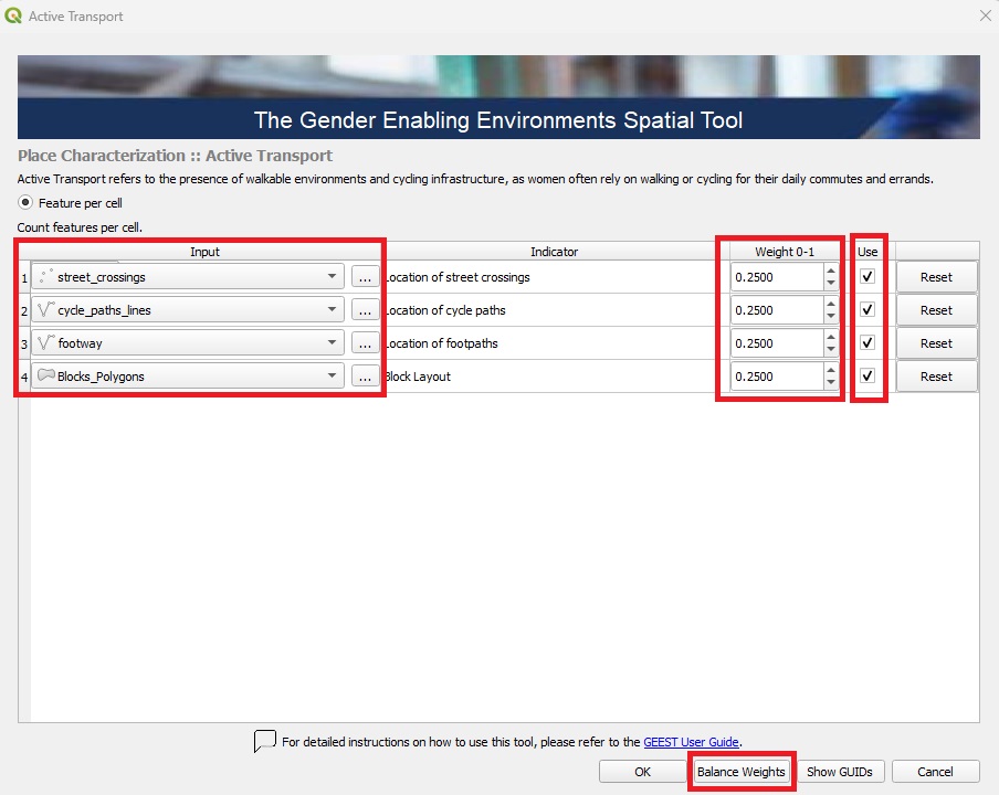
Active transport factor is calculated based on the four subfactors averaged across the raster cells:
Subfactor |
Score 0 |
Score 1 |
Score 2 |
Score 3 |
Score 4 |
Score 5 |
|---|---|---|---|---|---|---|
Street Crossings |
None |
N/A |
N/A |
1 crossing |
N/A |
2+ crossings |
Cycle Paths |
None |
N/A |
N/A |
1 cycle path |
N/A |
2+ paths |
Footpaths |
None |
N/A |
N/A |
1 path |
N/A |
2+ paths |
Block Sizes |
None |
>1 km |
751m - 1 km |
501m - 750m |
251m - 500m |
<250m |
Process Active Transport factors
Back in the Data Processing Interface:
🖱️ Right-click on Active Transport.
▶️ Select “Run Item Workflow” from the context menu to initiate the process.

The successful completion of the process is indicated by the green checkmark widgets.
Safety#
Safety addresses the perceived security of public spaces, evaluated through the availability of adequate lighting, which affects women’s ability to move freely, seek employment, and access essential services.
Locate Safety Section
🖱️🖱️ Double-click on the Safety section to open the pop-up.
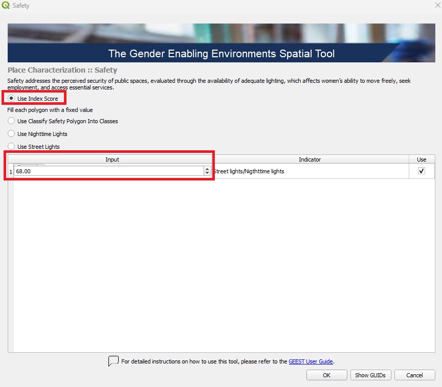
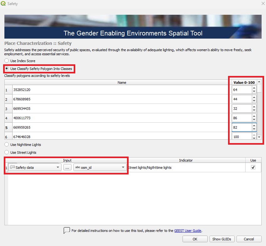
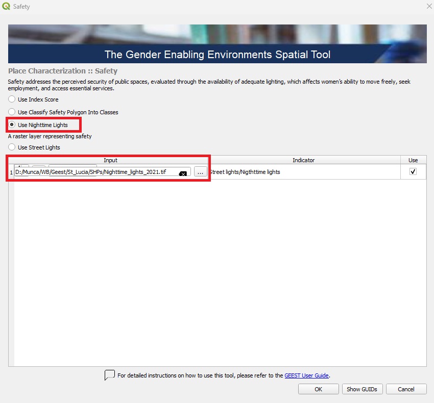
📂 Flexible Data Input Options: Multiple data input options are available depending on the data’s availability, format, or geographic coverage. Select one of the following options:
1️⃣ Using Perceived Safety data index score as input:
2️⃣ Using Classified Safety data as input; select the layer already loaded in the QGIS Layer Panel from the dropdown menu or manually enter the file path for the shapefiles (polygon features) corresponding to the safety data by clicking the three-dot button and the classification field; this layer will be used for processing:
3️⃣ Using Nighttime Lights data as input; VIIRS Nighttime Lights raster may be used as proxy data for presence of area illumination at night time; select the layer already loaded in the QGIS Layer Panel from the dropdown menu or manually enter the file path for the (raster data) corresponding to NTL by clicking the three-dot button; this layer will be used for processing:
4️⃣ Using Street lights data as input; select the layer already loaded in the QGIS Layer Panel from the dropdown menu or manually enter the file path for the shapefiles (point locations) representing street lights by clicking the three-dot button; this layer will be used for processing:
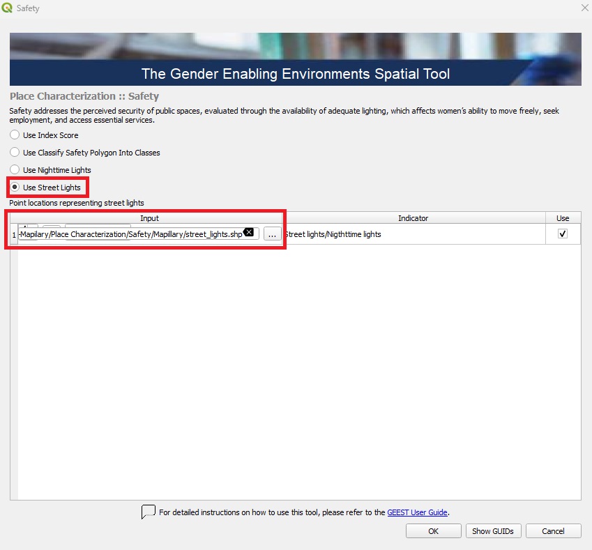
🚫 Exclude Unused Factors (optional): If this factor is not intended to be included in the process, uncheck the Use button associated with it.
✅ Finalize: Once all settings are configured, click OK to confirm and proceed to the next step.
Safety is calculated by generating 20-meter buffers around streetlights using the default thresholds:
Factor |
Score 0 |
Score 1 |
Score 2 |
Score 3 |
Score 4 |
Score 5 |
|---|---|---|---|---|---|---|
Safety |
No overlap |
1-19% intersection |
20-39% intersection |
40-59% intersection |
60-79% intersection |
80-100% intersection |
Note: Use nighttime light data only if streetlight data is unavailable.
Process Safety factor
Back in the Data Processing Interface:
🖱️ Right-click on Safety.
▶️ Select “Run Item Workflow” from the context menu to initiate the process.

The successful completion of the process is indicated by the green checkmark widgets.
FCV#
Fragility, conflict and violence (FCV) considers the frequency of events related to political unrest, conflict, and violence in a region, which can increase women’s vulnerability and limit their access to employment and essential services.
Locate FCV Section
🖱️🖱️ Double-click on the FCV section to open the pop-up.
📂 Flexible Data Input Options: Multiple data input options are available depending on the data’s availability, format, or geographic coverage. Select one of the following options:
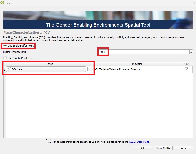
1️⃣ Using Point features data as input; select point locations representing data related to fragility, conflict and violence events; a buffer is needed to estimate the spatial impact of these events, the default radius is 5000m but if the impact radius of an event is known, it should be used instead:
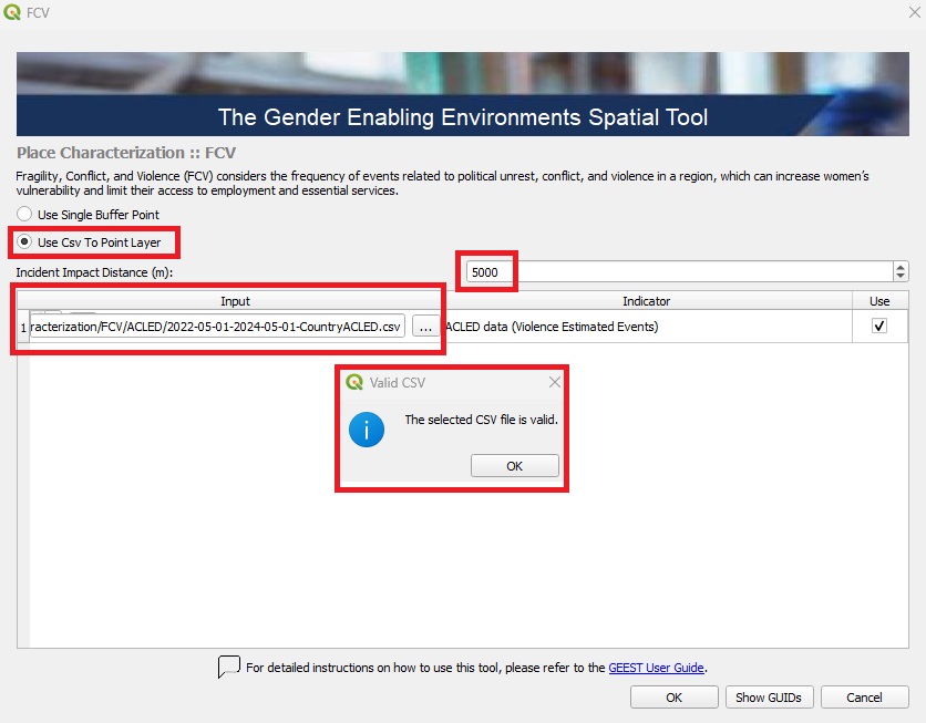
2️⃣ Using ACLED data as input; select ACLED data in CSV format representing fragility, conflict, and violence events; this indicator is structured by assigning scores to rasters based on their overlap with buffers indicating different types of events. Using point locations of FCV events, generate circular buffers with a default radius of 5 km to estimate the spatial impact of these events. If the impact radius of an event is known, it should be used instead; a pop-up will appear to validate the CSV format.
🚫 Exclude Unused Factor (optional): If this factor is not intended to be included in the process, uncheck the Use button associated with it.
✅ Finalize: Once all settings are configured, click OK to confirm and proceed to the next step.
FCV is structured by assigning scores to raster cells based on their overlap with buffers representing different types of events. Using point locations of FCV (Fragility, Conflict, and Violence) events, create circular buffers with a radius of 5 km to estimate the spatial impact. If a specific event’s impact radius is known, it should be applied instead. Raster cells intersecting with these default buffers are scored as follows:
Factor |
Score 0 |
Score 1 |
Score 2 |
Score 3 |
Score 4 |
Score 5 |
|---|---|---|---|---|---|---|
FCV |
battles and explosions |
explosions and remote violence |
violence against civilians |
not applicable |
protests and riots |
no overlap with any event |
Process FCV factor
Back in the Data Processing Interface:
🖱️ Right-click on FCV.
▶️ Select “Run Item Workflow” from the context menu to initiate the process.

The successful completion of the process is indicated by the green checkmark widgets.
Education#
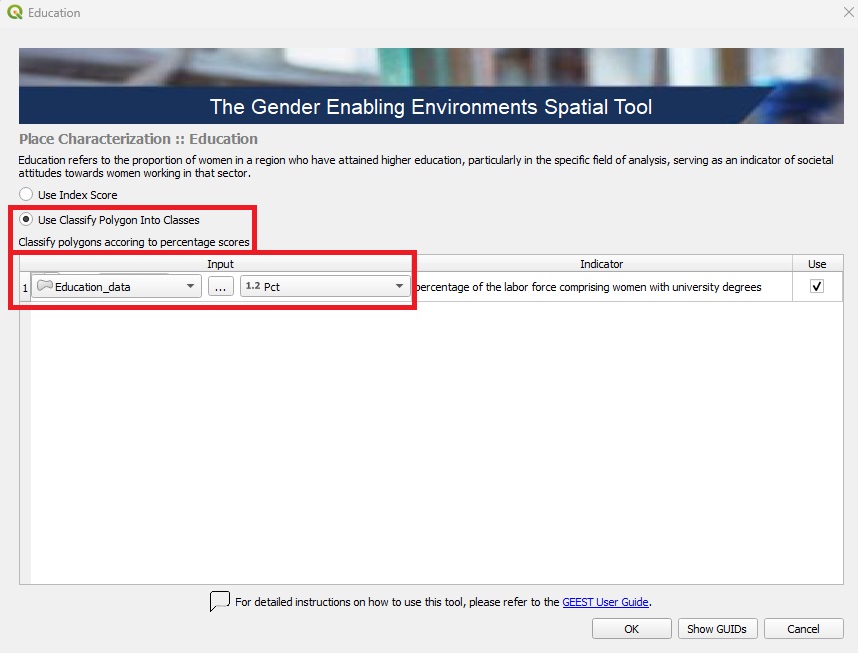
Education refers to the proportion of women in a region who have attained higher education, particularly in the specific field of analysis, serving as an indicator of societal attitudes towards women working in that sector.
Locate Education Section
🖱️🖱️ Double-click on the Education section to open the pop-up.
📂 Flexible Data Input Options: Multiple data input options are available depending on the data’s availability, format, or geographic coverage. Select one of the following options:
1️⃣ Using Index score at the national or regional level, based on the proportion of women who have attained higher education as input:
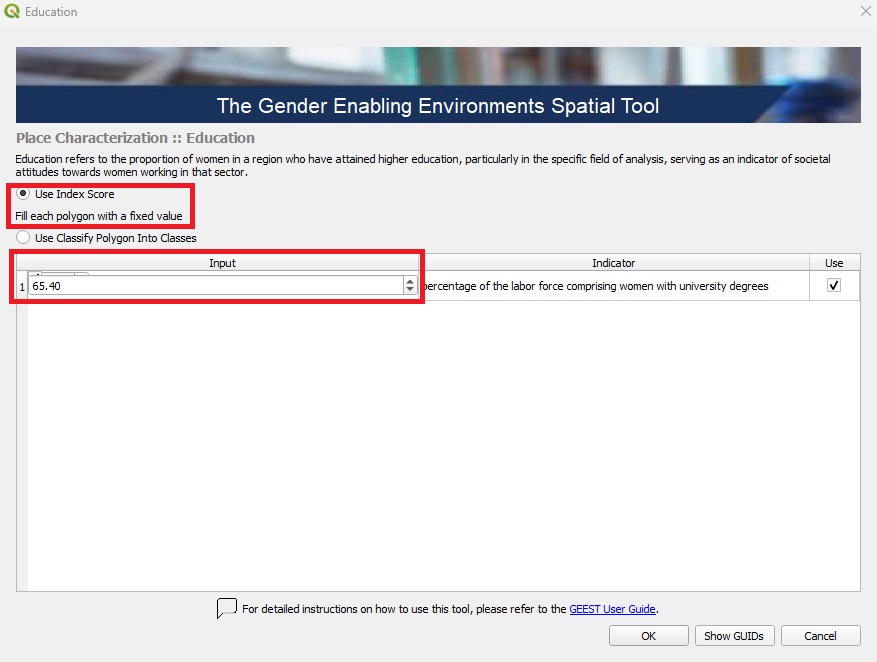
2️⃣ Using Classify Polygon Into Classes data as input; select the layer already loaded in the QGIS Layer Panel from the dropdown menu or manually enter the file path for the shapefiles (polygon features) corresponding to the education data by clicking the three-dot button then, select the classification field to be used for processing:
🚫 Exclude Unused Factor (optional): If this factor is not intended to be included in the process, uncheck the Use button associated with it.
✅ Finalize: Once all settings are configured, click OK to confirm and proceed to the next step.
Education reclassifies the input data to a standardized scale from 0 to 5 using a linear scaling process. In this scale, a score of 5 represents areas where all women have a university degree, while a score of 0 represents areas where no women have a university degree.
Process Education factor
Back in the Data Processing Interface:
🖱️ Right-click on Education.
▶️ Select “Run Item Workflow” from the context menu to initiate the process.

The successful completion of the process is indicated by the green checkmark widgets.
Digital Inclusion#
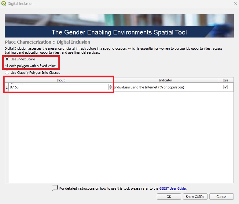
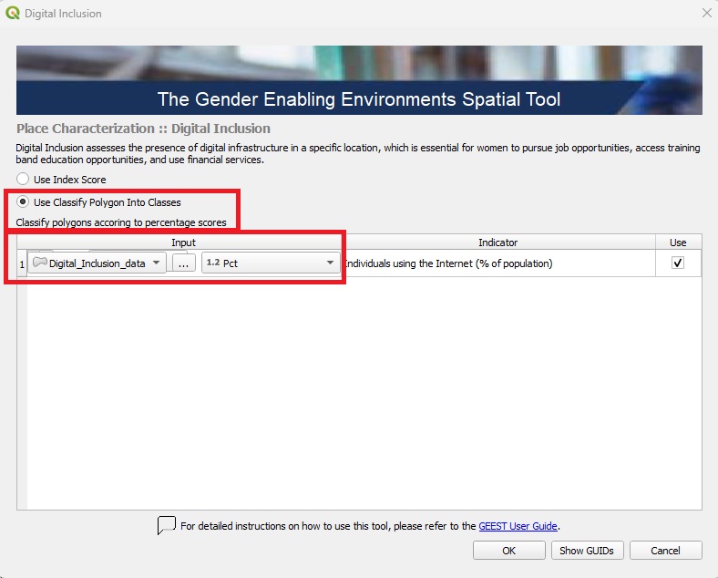
Digital Inclusion assesses the presence of digital infrastructure in a specific location, which is essential for women to pursue job opportunities, access training and education opportunities, and use financial services.
Locate Digital Inclusion Section
🖱️🖱️ Double-click on the Digital Inclusion section to open the pop-up.
📂 Flexible Data Input Options: Multiple data input options are available depending on the data’s availability, format, or geographic coverage. Select one of the following options:
1️⃣ Using Index score at the national or regional level, based on the proportion of available digital infrastructure as input:
2️⃣ Using Classify Polygon Into Classes data as input; select the layer already loaded in the QGIS Layer Panel from the dropdown menu or manually enter the file path for the shapefiles (polygon features) corresponding to the digital inclusion data by clicking the three-dot button then, select the classification field to be used for processing:
🚫 Exclude Unused Factor (optional): If this factor is not intended to be included in the process, uncheck the Use button associated with it.
✅ Finalize: Once all settings are configured, click OK to confirm and proceed to the next step.
Digital Inclusion reclassifies input data to a standardized scale of 0 to 5 using a linear scaling process, where 5 represents areas where 100% of households have internet access, and 0 represents areas where no households have internet access.
Process Digital Inclusion factor
Back in the Data Processing Interface:
🖱️ Right-click on Digital Inclusion.
▶️ Select “Run Item Workflow” from the context menu to initiate the process.

The successful completion of the process is indicated by the green checkmark widgets.
Environmental Hazards#
Environmental Hazards relate to the impact of environmental risks, such as floods, droughts, landslides, fires and extreme weather events, which can disrupt job stability, particularly for women in vulnerable sectors.
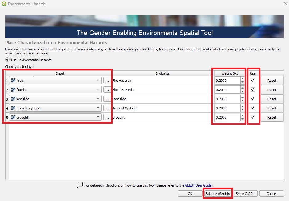
This factor is composed, by default, of five subfactors representing different types of hazards: fires, floods, landslides, tropical cyclones and droughts. These subfactors are aggregated into a single factor, referred to as Environmental Hazards, based on the selected weights assigned to each subfactor.
If data for one or more hazard types is not available, these subfactors can be excluded from the processing. In such cases, the tool will automatically adjust the weights of the remaining subfactors to ensure accurate aggregation.
The thresholds for defining hazard levels are based on a predefined scoring list. The input data relies on globally available open data sources and is reclassified for use within the tool. However, if more precise and localized data is available, users are encouraged to incorporate it into the processing. In doing so, users should align the data with the thresholds provided to maintain consistency and reliability.
Locate Environmental Hazards Section
🖱️🖱️ Double-click on the Environmental Hazards section to open the pop-up.
📝 In the Input field, you can select layers already loaded in the QGIS Layer Panel from the dropdown menu or manually enter the file path for the raster features corresponding to the indicators by clicking the three-dot button.
⚖️ Assign Weights: Assign appropriate weights to reflect the relative importance of each factor in the analysis. Ensure these values are consistent with your project objectives, accurately represent the significance of each factor and add up to 1 for a balanced evaluation.
🚫 Exclude Unused Factors (optional): If a specific factor is not intended to be included in the process, uncheck the Use button associated with it.
🔄 Readjust Weights: After excluding any factors, make sure to Balance Weights of the remaining factors. This step ensures the weight distribution remains balanced and totals correctly, preserving the integrity of the analysis.
✅ Finalize: Once all settings are configured, click OK to confirm and proceed to the next step.
Environmental Hazards reclassifies input data to a standardized scale of 0 to 5 using a linear scaling process, where 5 represents areas with no environmental hazards and 0 represents areas with the highest level of hazard.
Factor |
Class 0 |
Class 1 |
Class 2 |
Class 3 |
Class 4 |
Class 5 |
|---|---|---|---|---|---|---|
Number of Fires per km² |
>8 |
5–8 |
2–5 |
1–2 |
0–1 |
0 or No Data |
Floods Data |
720–900 cm |
540–720 cm |
360–540 cm |
180–360 cm |
<180 cm |
No Data or 0 |
Landslide Data |
Severe |
High-Moderate2 (4) |
Moderate (3) |
Low-Moderate1 (2) |
Slight (1) |
No Data or 0 |
Tropical Cyclone Frequency (100 Years) |
>100 events |
75–100 events |
50–75 events |
25–50 events |
<25 events |
No Data or 0 |
Drought Data |
4–5 |
3–4 |
2–3 |
1–2 |
0–1 |
No Data or 0 |
Process Environmental Hazards factors
Back in the Data Processing Interface:
🖱️ Right-click on Environmental Hazards.
▶️ Select “Run Item Workflow” from the context menu to initiate the process.

The successful completion of the process is indicated by the green checkmark widgets.
Water sanitation#
Water sanitation concerns the availability of clean water and sanitation facilities, affecting women’s time allocation and capacity to engage in employment.
Locate Water sanitation Section
🖱️🖱️ Double-click on the Water sanitation section to open the pop-up.
📝 In the Input field, you can select layers already loaded in the QGIS Layer Panel from the dropdown menu or manually enter the file path for the shapefiles (point features) corresponding to the water and sanitation facilities by clicking the three-dot button; a buffer is needed to estimate the spatial impact of these facilities, the default radius is set to 1000 meters; however, this value can be adjusted based on the user’s considerations.
🚫 Exclude Unused Factor (optional): If this specific factor is not intended to be included in the process, uncheck the Use button associated with it.
✅ Finalize: Once all settings are configured, click OK to confirm and proceed to the next step.
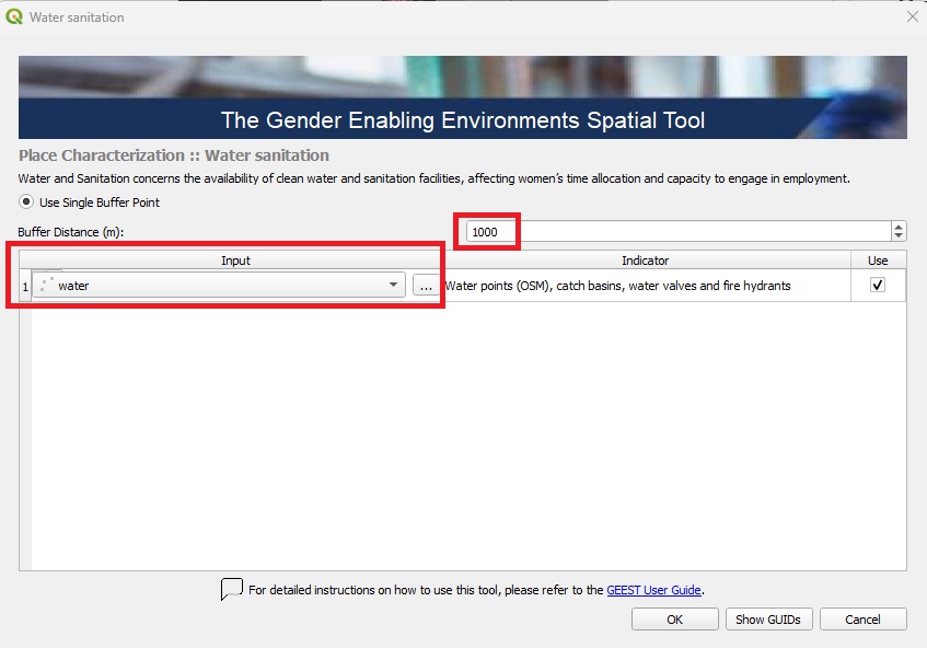
Water Sanitation is assessed based on the presence of water and sanitation facilities within a raster cell, applying a default 1000m buffer. The scoring is as follows:
Factor |
Score 0 |
Score 1 |
Score 2 |
Score 3 |
Score 4 |
Score 5 |
|---|---|---|---|---|---|---|
Water Sanitation |
No water points |
N/A |
N/A |
1 water point |
N/A |
2 or more water points |
Process Water sanitation factor
Back in the Data Processing Interface:
🖱️ Right-click on Water sanitation.
▶️ Select “Run Item Workflow” from the context menu to initiate the process.

The successful completion of the process is indicated by the green checkmark widgets.
Additional Steps Before Processing:
🖱️🖱️ Double-click on the Place Characterization section to open the pop-up.
⚖️ Assign Weights: Ensure the weights are correctly assigned, as they determine the relative importance of each factor in the analysis. Carefully review these values to ensure they are aligned with your project’s objectives and reflect the significance of each factor accurately.
🚫 Exclude Unused Factors (optional): If a specific factor is not intended to be included in the process, uncheck the Use button associated with it.
🔄 Readjust Weights: After excluding any factors, make sure to Balance Weights of the remaining factors. This step ensures the weight distribution remains balanced and totals correctly, preserving the integrity of the analysis, then click OK to proceed.
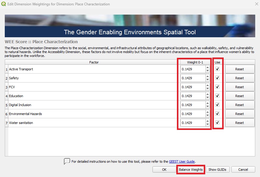
Process Place Characterization factors#
After configuring the factors and adjusting their weights to achieve balance, you can initiate the process workflow:
🖱️Right-click on Place Characterization.
▶️Select Run Item Workflow from the context menu.
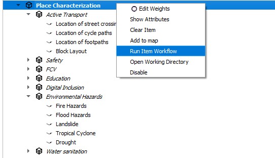
The process should be successfully completed and indicated by a green checkmark widget.
Visualizing the Outputs#
After completing the process, the outputs are automatically added to the Layer Panel in QGIS as a group layer. This group layer has the Mutually Exclusive Group feature activated, which ensures that only one layer within the group can be visible at a time. When this feature is enabled, turning on the visibility of one layer automatically turns off the visibility of the others within the same group, making it easier to compare results without overlapping visualizations.
The outputs consist of all factors and subfactors, as well as the aggregation of these into the final Place Characterization output. All scores are assessed on a scale from 0 to 5, categorized as follows: ≤ 0.5 (Not Enabling) | 0.5–1.5 (Very Low Enablement) | 1.5–2.5 (Low Enablement) | 2.5–3.5 (Moderately Enabling) | 3.5–4.5 (Enabling) | 4.5–5.0 (Highly Enabling).
The outputs are stored under the Place Characterization folder within the project folder created during the setup phase as raster files. These files can be shared and further utilized for various purposes, such as visualization in QGIS or other GIS software, integration into reports, overlaying with other spatial datasets, or performing advanced geospatial analyses, such as identifying priority areas or conducting trend analysis based on the scores.
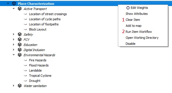
If the results do not immediately appear in the Layer Panel after processing the Place Characterization Dimension, you can resolve this by either adding them manually from the folder path or by right-clicking on the Place Characterization Dimension and selecting Add to map from the context menu:
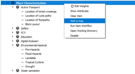
💡 Tip: If the input needs to be changed for any reason (e.g., incorrect initial input), you can clear the results and reprocess them as follows:
🖱️ Right-click on the factor/dimension and select Clear Item.
🖱️ Right-click again on the same cleared factor/dimension, and while holding the SHIFT key on your keyboard, select Run Item Workflow. This process ensures that the tool reassesses the input datasets and outputs the corrected scores.
Key Considerations#
Input Accuracy: Ensure all input datasets are carefully entered/selected and correspond to the correct factors and/or subfactors. Incorrect data will impact the outputs and subsequent analysis.
Weight Adjustment: Assign weights thoughtfully to reflect the importance of each factor in the overall analysis. After making changes, always balance the weights to ensure they sum up correctly.
