Data Governance Principles
Raw data (SharePoint) | Code (git+GitHub) | Results (disposable|local or shared)
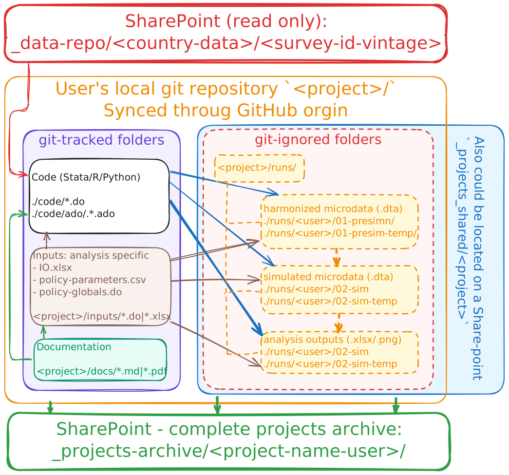
If you remember only one sentence: raw data is an input you never touch, results are an output you can always throw away and reproduce, and everything in between is code under version control.
Principle 1: raw data lives outside the code
Raw data sits on SharePoint, read-only, in
_data-repo/.Code sits on GitHub, in
github.com/worldbank/your_repo: GitHub is a source of truth!The two are joined at run time by a path global: never by copying data into the repository.
- Any
code - Analysis-specific inputs that are assumptions chosen by the analyst, not observations.
- Template excel dashboard for the client
- copied to the results at the analysis stage and populated with the results data.
- Any number that could be followed by “why is this chosen?”, e.g., poverty lines, conversion rates, equivalence scales
- Scenario definitions
- Concordance and mapping tables (sector crosswalks, region recodes, etc.)
- Files must be small (<5–10 MB), text-based, human-readable diff (
.csv,.do,.md,.yaml, etc.), free of personal data
Principle 2: results are disposable
Every file the analysis produces must be reproducible from the raw data by running the code — no matter how long the run takes and how many stages it has.
Delete the entire
runs/folder, run00_master.do, and get your results back.: Nothing produced is precious.Raw and inputs are never written to.
- Have an excel dashboard? Copy it to
runs/and populate it there. Do not edit the template ininputs/.
- Have an excel dashboard? Copy it to
Manual edits are not allowed.
- Need to fix the excel dashboard? Edit it in
inputs/.
- Need to fix the excel dashboard? Edit it in
Disposability is about the working life of a project, not about the record. When a project is delivered, a dated, self-contained copy — raw data, code, inputs, and the outputs actually shown to the client — is deposited in _projects-archive/ and stops changing. The two rules do not conflict: you archive a snapshot precisely because the live folder is meant to be thrown away and rebuilt.
Principle 3: Any data pipeline has three stages
Every MML analysis runs in the same three stages, in this order.
| Stage | File | Reads | Produces |
|---|---|---|---|
| Pre-simulation | XX_presim.do |
the raw archive (the only stage that may) | harmonised, analysis-ready micro data |
| Simulation | YY_sim.do |
the pre-sim product (never from the raw archive) | simulated household-level data |
| Post-simulation | ZZ_postsim.do |
the sim product (never from the raw archive or presim) | indicators, tables, figures, dashboards |
Two rules make the stages worth having.
- Each stage reads only its predecessor’s product.
- Each stage hands off through a folder on disk, not through memory.
Why this particular cut:
Pre-sim where all source-specific decisions live — variable names, value labels, missing codes, deflators, survey quirks. Isolating them means swapping a country or a survey round touches one file.
Sim where the method lives. It sees a clean, standard dataset, knows nothing about where it came from, but knows everything about how it should be transformed.
Post-sim where the presentation lives: tables, figures, dashboard (.xlsx/shiny). It never recomputes the simulation, so a formatting change can never move a number.
Where these three principles come from?
None of this is invented here. Founding principals are coming from:
- ETL/ELT/ data pipelines
- Medallion Architecture (bronze → silver → gold)
- Coockiecutter Data Science
ETL/ELT
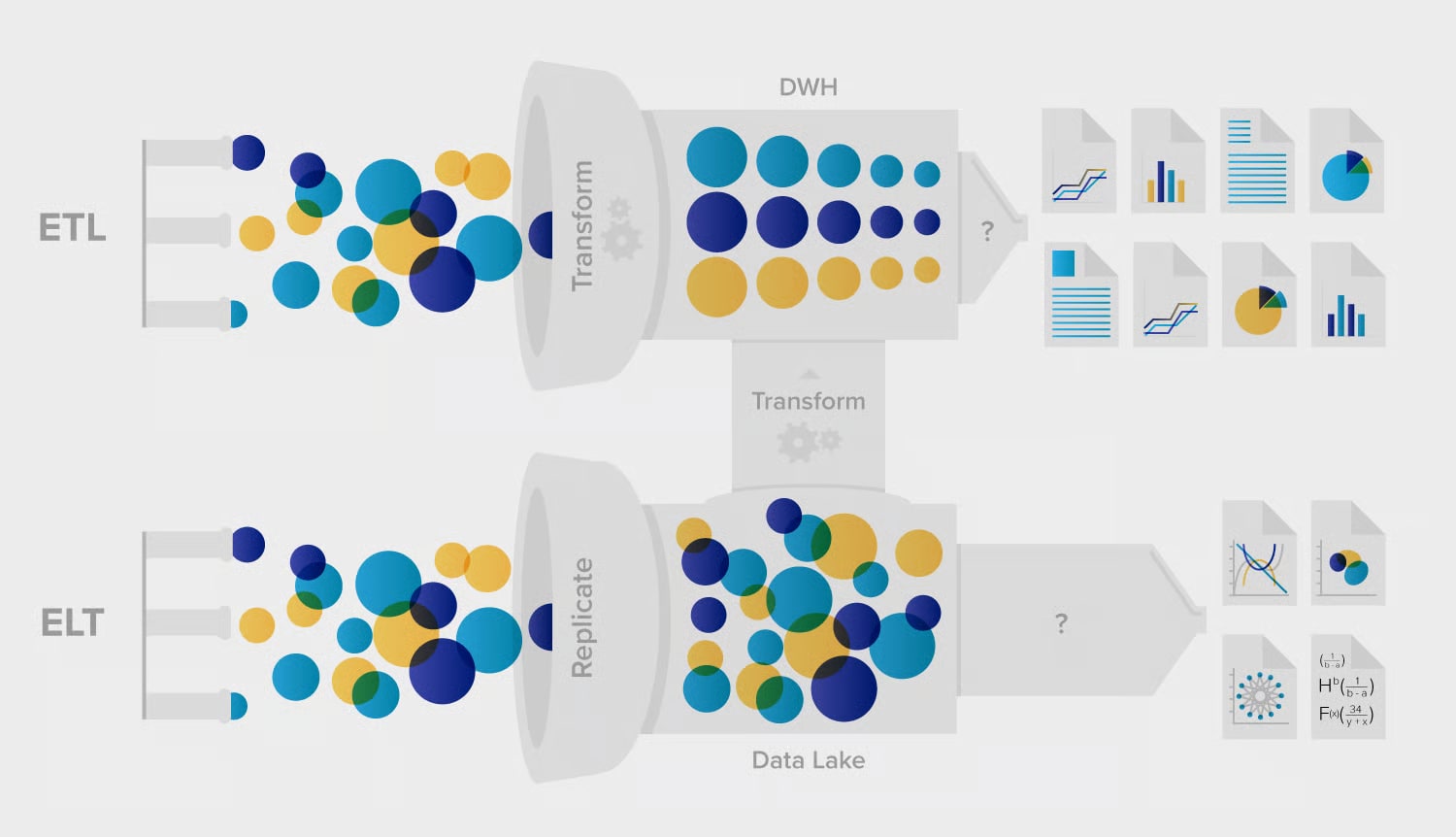
Every data pipeline does the same three things in a different order:
- extract data from its sources,
- transform it into an analysis-ready shape, and
- load it into wherever the analysis happens.
ETL transforms the data before it is saved in operational format; ELT loads the raw data first and transforms it afterwards on the fly.
Our three principles are ELT, done in Stata.
- extract: depositing raw data from SharePoint;
- load: read-only archive - never written to.
- transform:
pre-sim,simandpost-simeverything downstream of the archive is derived by code and can be rebuilt from scratch.
ETL — extract, transform, load
Data is pulled from the sources, cleansed, standardised, aggregated and enriched in a staging area, and only the finished product is written into the target data warehouse.
Pros
- Consistency, quality and security are enforced before anything lands.
- Sensitive fields can be masked or encrypted on the way in — good for compliance.
- Keeps the transformation load off the target system.
- Fits smaller sources with complex transformation logic.
- Granular control over every step of the process.
Cons
- Slower ingestion overall.
- Extra processing overhead in the intermediary system.
- Hard to scale to very large data without buying infrastructure.
- The transformation is fixed up front: a new question means re-running the pipeline.
ELT — extract, load, transform
Data is pulled from the sources and written into the target — a warehouse or a data lake — untouched, and the transformations are run inside the target afterwards.
Pros
- Flexible: the transformation logic can be decided, and changed, after loading.
- Faster ingestion, because the data moves once.
- Uses the massively parallel compute of the target system.
- More efficient for very large datasets.
- Adapts quickly when the question changes.
Cons
- Raw, unmasked data sits in the target until the transformations are done — a compliance risk.
- Depends on what the target system can do, rather than on your own tooling.
- Less granular control during the transformation phase.
- A poor fit where data-handling rules are strict.
Medallion Architecture
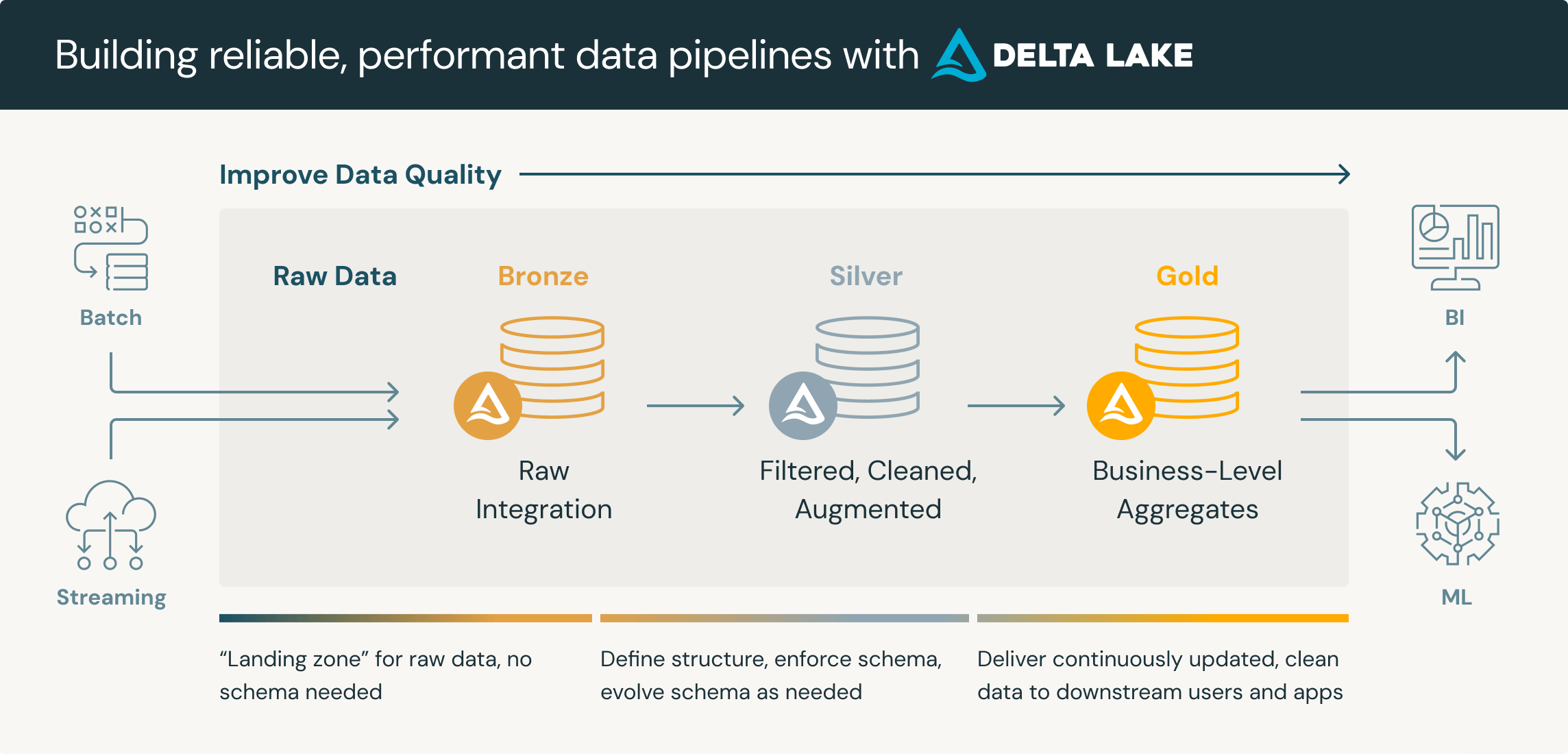
Medallion architecture organises data in three layers that progressively improve its structure and quality:
bronze holds every source’s data exactly as it arrived, plus load metadata, and acts as the historical archive from which anything downstream can be rebuilt without going back to the source;
silver is the cleaned, filtered and conformed view of that data, standardised across sources and fit for general use;
gold is read-optimised, project-specific output — the aggregates, indicators and tables actually consumed by reports and models.
Our pre-sim, sim and post-sim are the same three tiers under different names, and they are cut this way for the same reason: because each layer is derived from the one before it, you can always throw the later ones away and recreate them.
The post-simulation stage of the Fiscal Incidence Analysis developed by Pechi and colleagues follows the bronze-silver-gold layer pattern.
Other literature
The three principles are the standard reproducibility practice of empirical economics and of data engineering generally, stated in MML’s vocabulary.
| Source | What it says that matches |
|---|---|
| Wilson et al. (2017), Good Enough Practices in Scientific Computing | Literally our Principles 1 and 2: “save the raw data”, “treat data as read-only”, “treat generated output as disposable” |
| Gentzkow & Shapiro (2014), Code and Data for the Social Sciences | Automate everything; one script runs the whole project end to end; separate directories by function and separate inputs from outputs |
| Bjärkefur et al. (2021), Development Research in Practice (DIME Analytics, World Bank) | The same pipeline, cut into four: acquisition → processing → construction → analysis. Our pre-sim covers processing and construction; sim and post-sim split their analysis step |
| Cookiecutter Data Science | “Data is immutable”; data/raw is never edited; the analysis is a directed graph from raw to results |
| Medallion / lakehouse architecture (bronze → silver → gold) | The same three tiers in engineering language: immutable landing zone, conformed data, presentation-layer aggregates |
| Wilkinson et al. (2016), FAIR principles | Findable, Accessible, Interoperable, Reusable — the metadata and documentation side of the archive readme.md requirement |
| World Bank Reproducible Research Repository | The delivery-time test: a third party re-runs the package from scratch and gets the same numbers |