6. Expressions (continued)¶

# reminder that if you are installing libraries in a Google Colab instance you will be prompted to restart your kernal

try:
    import geemap, ee
except ModuleNotFoundError:
    if 'google.colab' in str(get_ipython()):
        print("package not found, installing w/ pip in Google Colab...")
        !pip install geemap
    else:
        print("package not found, installing w/ conda...")
        !conda install mamba -c conda-forge -y
        !mamba install geemap -c conda-forge -y
    import geemap, ee

try:
        ee.Initialize()
except Exception as e:
        ee.Authenticate()
        ee.Initialize()

# # initialize our map and center on Mexico City, Mexico
lat = 19.43
lon = -99.13

# get 1996 composite, apply mask, and add as layer
dmsp1996 = ee.Image("NOAA/DMSP-OLS/NIGHTTIME_LIGHTS/F121996").select('stable_lights')
dmsp1996_inv = dmsp1996.multiply(-1).add(63)

6.1. Invert image with `.expression()`¶

Now, we’ll perform the same operation as we did before, but using the expression() method.

The ee.Image.expression() method takes a string input as the formula. The second argument is a dictionary with key-value pairs, where the keys are the characters in our string we want to use as variables, (e.g. “X”) and the values are the corresponding data – a particular Image band in this case.

inv_formula = "(X*-1) + 63"

# we plug this formula in, identify our variable "X" and set it to our 1996 DMSP-OLS "stable_lights" band
dmsp1996_inv2 = dmsp1996.expression(inv_formula, {'X':dmsp1996})

6.1.1. Gut-check visualization…¶

If we inspected dmsp1996_inv and dmsp1996_inv2 analytically we’d see they were identical. For now, you can see visually that they are the same by comparing the two layers.

Warning, this is based on `ipyleaflet` a Python library that does not play well with Google Colab, so the split panel display will not work in the Google Colab environment but should on your local machine.

map1 = geemap.Map(center=[lat,lon],zoom=6)
map1.addLayerControl()

dmsp96inv_tile = geemap.ee_tile_layer(dmsp1996_inv, {'min':0,'max':63}, 'DMSP 96 inverse', opacity=0.75)
dmsp96inv_tile2 = geemap.ee_tile_layer(dmsp1996_inv2, {'min':0,'max':63}, 'DMSP 96 inverse 2nd method', opacity=0.75)


map1.split_map(left_layer=dmsp96inv_tile, right_layer=dmsp96inv_tile2)
map1

They’re equivalent!

So…why use the expression() method instead of the built-in functions?

This method used a couple very simple operations, but it can be necessary to use more complex formulae.

It can be easier to read an expression written in a form (like a string) that we’re familiar with. It may also be easier to dynamically update formulae with different variables when using the .expression() approach. We’ll show a practical use of this in DMSP-OLS intercalibration (10 min).

6.1.2. Apply a polynomial function to calibrate a DMPS-OLS image¶

We cover DMSP-OLS intercalibration in more detail in a later exercise, but as an illustrative example of expressions, we’re going to look at this intercalibration formula, which applies a series of coefficients to an input DMSP-OLS image to get an “adjusted” image that corrects for sensor variation (technical paper here [EZB+09]):

These coefficients map to the formula: \(X' = C_{0} + C_{1}*X + C_{2}*X^{2}\)

Where:

X: the input image, represented as a 2-dimensional matrix (recall these images are panchromatic so there is only one channel of light)
\(C_{0}, C_{1}, C_{2}\): the calibration coefficients that are assigned to each satellite
X’: the calibrated image

This is a table of the coefficients created using this method corresponding to specific DMSP-OLS satellite-year data:

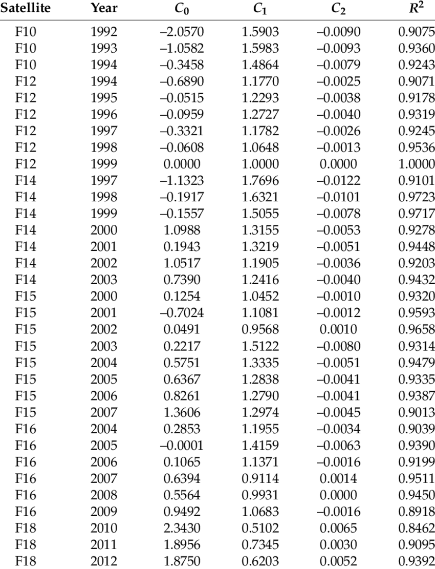
Fig. 6.1 DMSP-OLS intercalibration [JHL+17]¶

For 1996, there is only one satellite, F12, so we can reference the appropriate coefficients for F121996 from our table above:

\(C_{0}\) = -0.0959
\(C_{1}\) = 1.2727
\(C_{2}\) = -0.0040

We add our coefficients to the appropriate terms of the polynomial and set our input image as the X variable and save this formula as a string.

# set our formula
F121996cal = '-0.0959 + (1.2727 * X) + (-0.0040 * X * X)'

# apply our expression to our 1996 composite
# dmsp1996 = ee.Image("NOAA/DMSP-OLS/NIGHTTIME_LIGHTS/F121996").select('stable_lights')
dmsp1996_clbr = dmsp1996.expression(F121996cal,{'X':dmsp1996})

6.1.3. Visualize¶

Warning, this is based on `ipyleaflet` a Python library that does not play well with Google Colab, so the split panel display will not work in the Google Colab environment but should on your local machine.

map2 = geemap.Map(center=[lat,lon],zoom=9)
map2.addLayerControl()

mask96 = geemap.ee_tile_layer(dmsp1996.mask(dmsp1996), {'min':0,'max':63}, 'DMSP NTL 1996', opacity=0.75)
adj96 = geemap.ee_tile_layer(dmsp1996_clbr.mask(dmsp1996_clbr), {'min':0,'max':63}, 'DMSP NTL 1996 adjusted', opacity=0.75)

map2.split_map(left_layer=mask96, right_layer=adj96)
map2

6.1.4. A subtle adjustment…¶

Note that visually, the changes are hard to detect, but if you zoom in, you can see that the adjusted image has brighter values around the edges of the urban areas.

If we were actually conducting inter-calibration, we’d also clip the adjusted image to specific minimum and max values to account for the fact that some DN values are above our 63 max (you guessed it, more on that in a later exercise).

For now, you know how use .expression() to perform more complex operations on Images!

6.2. References:¶

EZB+09: Christopher D Elvidge, Daniel Ziskin, Kimberly E Baugh, Benjamin T Tuttle, Tilottama Ghosh, Dee W Pack, Edward H Erwin, and Mikhail Zhizhin. A fifteen year record of global natural gas flaring derived from satellite data. Energies, 2(3):595–622, 2009.
JHL+17: Wei Jiang, Guojin He, Tengfei Long, Chen Wang, Yuan Ni, and Ruiqi Ma. Assessing light pollution in china based on nighttime light imagery. Remote Sensing, 9(2):135, 2017.

Open Nighttime Lights