![]()
3. Introduction to Jupyter notebooks (10 min)
Jupyter notebooks have gained a lot of popularity in the scientific computing community, largely because of the ease with which users can integrate executable code with written text and plots interactively, making it a powerful tool for conducting data exploration and communicating analytical insights.
3.1. Getting started
Per Getting started with Python (10 min) you should already have jupyter installed in your environment.
By default the notebook uses a Python kernel (whatever Python version is in your current environment), so we dont need to worry about changing the language since we’re working in Python.
First, activate your virtual environment by opening a CLI (terminal) window (remember we named our environment “onl”):
$ conda activate onl
Now within your active environment, enter:
$ jupyter notebook
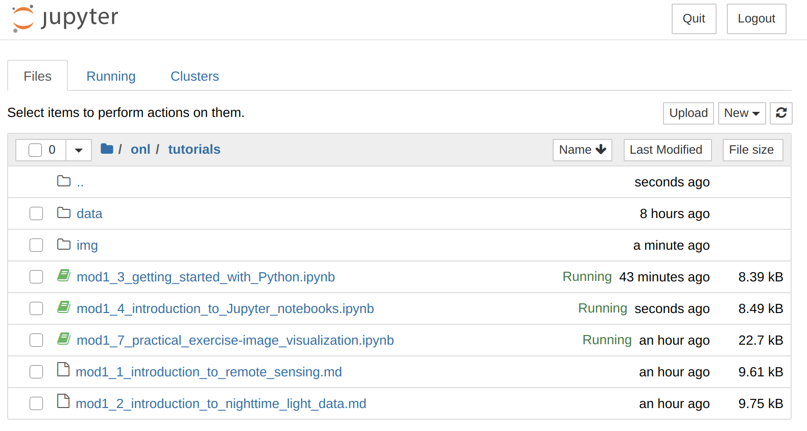
This launches the web server and your default browser (Chrome, Safari, Firefox, etc.) will open a tab showing a file directory based on your current location Fig. 3.1. You can navigate to existing notebook files (which contain the .ipynb extension) and open them in a new tab simply by clicking on them.
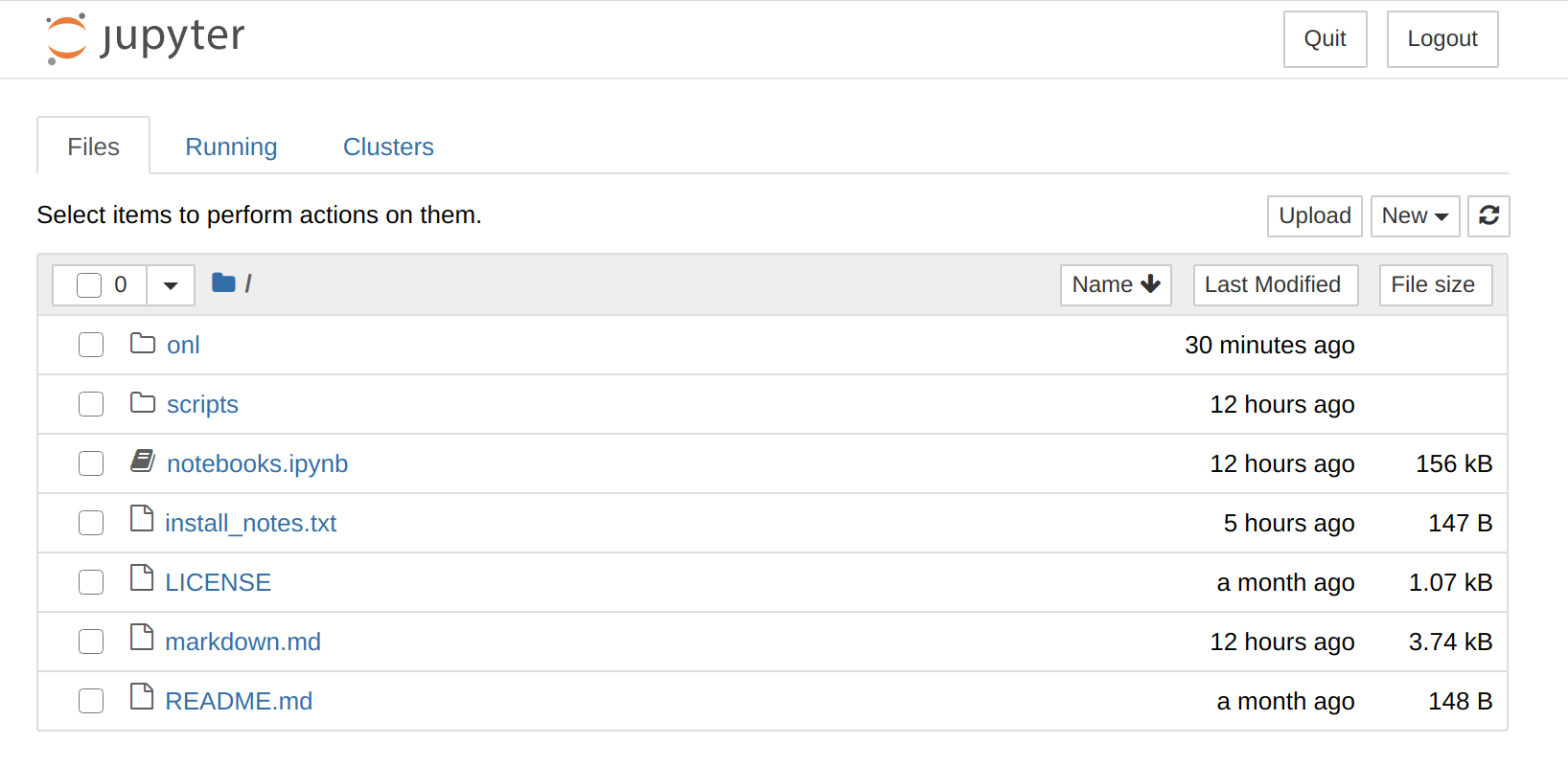
Fig. 3.1 Jupyter tree
We encourage you to explore the documentation and examples to see what is capable with Jupyter notebooks. Here, we’ll just cover some basic concepts that allow you to use this tutorial.
As noted, Jupyter notebooks contain cells. You can select what sort of content the cell contains, such as markdown text or executable code.
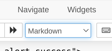
Fig. 3.2 Select the type of cell you want, e.g. markdown or code.
This very text you’re reading now is actually a markdown cell in a notebook.
And here is an example of executable code which produces an output:
print("hello world")
hello world
Which you could also wrap in a simple function and define that in one cell:
def sayHello():
    print("hello world")
…And then execute in a later cell:
sayHello()
hello world
The menu bar provides an option to run the cell (keyboard shortcut: SHIFT + ENTER). You can also run all the cells in the notebook.
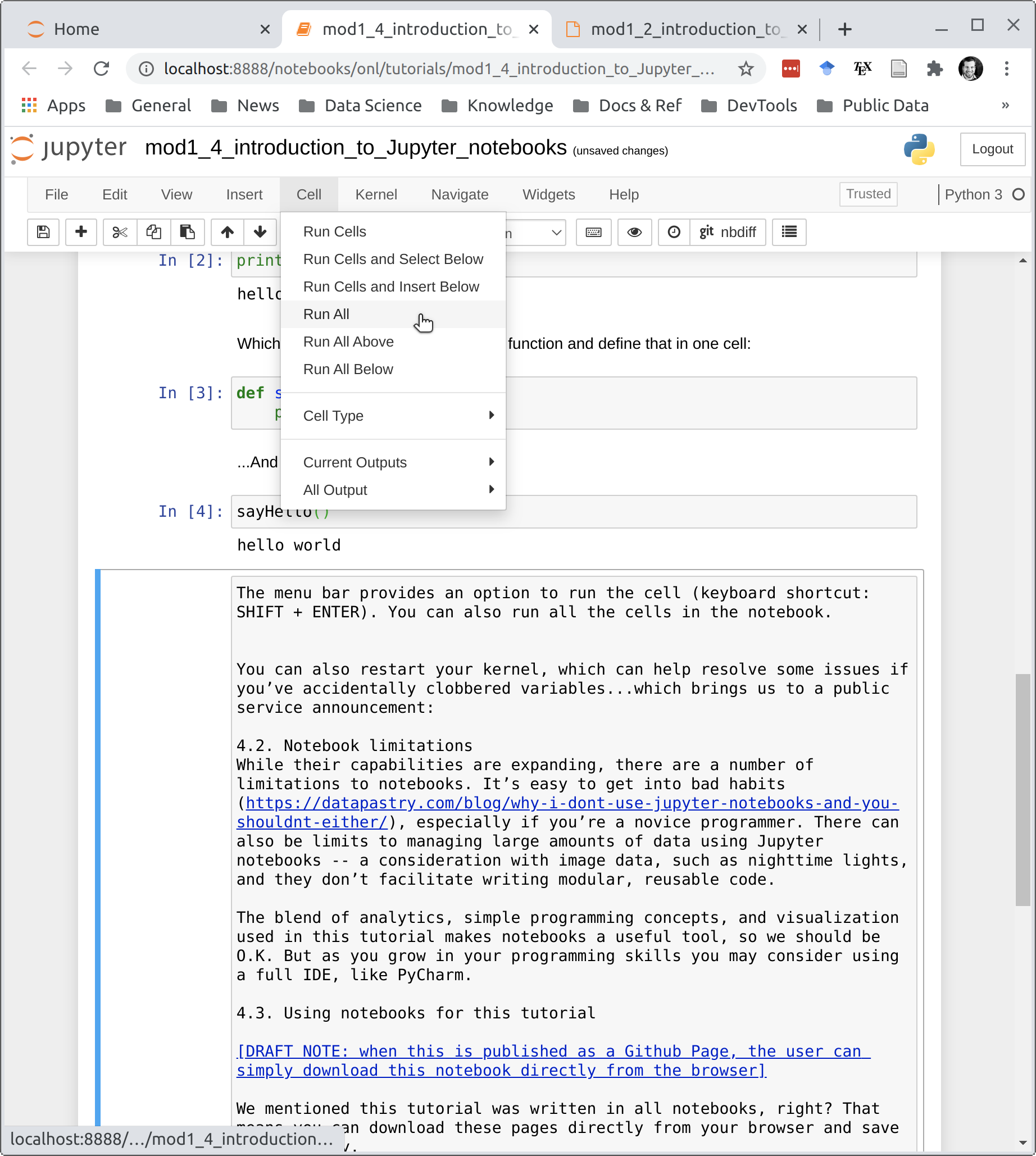
Fig. 3.3 Running cells independently allows for interactive code execution that can be useful for exploring and plotting data.
You can also restart your kernel:
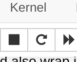
Fig. 3.4 Warning: restarting your kernel resets your memory, so you’ll lose all created variables and dump any data loaded in memory.
Restarting can help resolve some issues if you’ve accidentally clobbered variables….which brings us to a public service announcement:
3.1.1. Notebook limitations
While their capabilities are expanding, there are a number of limitations to notebooks. It’s easy to get into bad habits, especially if you’re a novice programmer. There can also be limits to managing large amounts of data using Jupyter notebooks – a consideration with image data, such as nighttime lights, and they don’t facilitate writing modular, reusable code.
The blend of analytics, simple programming concepts, and visualization used in this tutorial makes notebooks a useful tool, so we should be O.K. But as you grow in your programming skills you may consider using a full IDE, like PyCharm.
3.2. Using notebooks for this tutorial
We mentioned this tutorial was written in notebooks, right? That means you can download these pages directly from your browser and save them locally.
To do this
open your terminal in the directory where you want to work on this project
activate your virtual environment:
$ conda activate onllaunch a notebook instance like shown above:
$ jupyter notebook
Then, on this webpage, download this page as a notebook (.ipynb extension) and save it within the directory you launched the notebook from. You can do this from the icon at the upper right-hand side of this page:
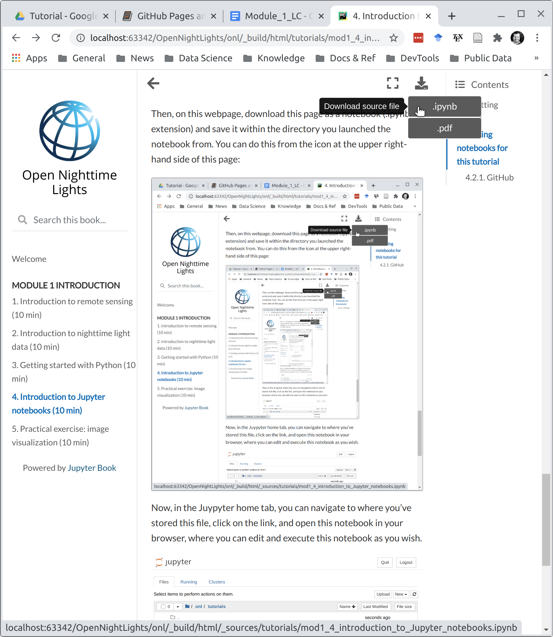
Now, in the Jupyter home tab, you can navigate to where you’ve stored this file, click on the link, and open this notebook in your browser, where you can edit and execute this notebook as you wish.
3.3. Google Colab notebooks
In addition to using Jupyter notebooks on your local machine, Google Colab is a helpful platform. By hosting notebooks on Google’s cloud infrastructure, you do not need to have your local computer set up with Python or any libraries and dependencies. You just need (good!) internet access and a Google account. You can also access computer processing resources, such as Graphics Processing Units (GPUs) for machine learning or image processing work.
PLEASE NOTE that due to the complex nature of interactive plots, some funcationality is limited in Colab. Also, conda is not installed natively and while we could install it, it is easier to use pip for Colab, so our import method will use pip as package manager rather than conda.