Tutorial, Module 3: Disruption#
This notebook is a template workflow to collect data and prepare the main data to perform a baseline physical accessibility analysis to health facilities. It uses various tools developed by the World Bank’s Geospatial Operations Support Team (GOST).
This notebook represents the third module of the tutorial on the physical accessibility to health facilities in a context of emergency.
It focuses on the datasets and the functions to be used to perform the analysis. A particular focus will be put on the uncertainty and pros&cons deriving from the utilization of different datasets. \
Setup#
Import packages required for the analysis
# System
import sys
import os
from os.path import join, expanduser
from pathlib import Path
# Avoid warnings to pop up
import warnings
warnings.filterwarnings('ignore')
# Visualization tools
# import folium as flm
import matplotlib.pyplot as plt
import matplotlib.colors as colors
import matplotlib.gridspec as gridspec
from rasterio.plot import plotting_extent
from rasterio.plot import show
from mpl_toolkits.axes_grid1 import make_axes_locatable
import contextily as ctx
import cartopy
import cartopy.crs as ccrs
import cartopy.feature as cfeature
import seaborn as sns

os.environ['CARTOPY_USER_BACKGROUNDS'] = '/home/jupyter-wb618081/Python/Backgrounds/'
# Processing
import numpy as np
import geopandas as gpd
import pandas as pd
from gadm import GADMDownloader
import dask_geopandas as dask_gpd

# Raster
import rasterio as rio
from rasterio.features import shapes
from shapely.geometry import box
from rasterio.features import geometry_mask
from rasterstats import zonal_stats
from shapely.geometry import Polygon, box, Point
from shapely.geometry import mapping
import skimage.graph as graph
from scipy.signal import convolve2d

# Graph
import pickle
import networkx as nx
import osmnx as ox

# for facebook data
from pyquadkey2 import quadkey
# Climate/Flood
# import xarray as xr
# Define your path to the Repositories

sys.path.append(join(expanduser("/home/jupyter-wb618081"), 'Repos', 'gostrocks', 'src'))
sys.path.append(join(expanduser("/home/jupyter-wb618081"), 'Repos', 'GOSTNets_Raster', 'src'))
sys.path.append(join(expanduser("/home/jupyter-wb618081"), 'Repos', 'GOSTnets'))
sys.path.append(join(expanduser("/home/jupyter-wb618081"), 'Repos', 'GOST_Urban', 'src', 'GOST_Urban'))
sys.path.append(join(expanduser("/home/jupyter-wb618081"), 'Repos', 'health-equity-diagnostics', 'src', 'modules'))
sys.path.append(join(expanduser("/home/jupyter-wb618081"), 'Repos', 'INFRA_SAP'))

import GOSTnets as gn
from GOSTnets.load_osm import *
import GOSTRocks.rasterMisc as rMisc
from GOSTRocks.misc import get_utm
import GOSTNetsRaster.market_access as ma
import UrbanRaster as urban

from infrasap import aggregator
from infrasap import osm_extractor as osm

from utils import download_osm_shapefiles
# auto reload
%load_ext autoreload
%autoreload 2
The autoreload extension is already loaded. To reload it, use:
  %reload_ext autoreload
Define below the local folder where you are located
scratch_dir = join(expanduser("/home/jupyter-wb618081"), 'Health-Access-Metrics', 'Tutorials')
data_dir = join(scratch_dir, 'tutorial_data')
out_path = join(scratch_dir, 'tutorial_output')
## Function for creating a path, if needed ##
def checkDir(out_path):
    if not os.path.exists(out_path):
        os.makedirs(out_path)
Data Preparation#
Import the City boundaries (.shp)#
epsg = "EPSG:4326"
epsg_utm = "EPSG:28232"
city = gpd.read_file((data_dir+"/brazaville.shp"))
city.to_crs(epsg)
city
| ID_0 | COUNTRY | NAME_1 | NL_NAME_1 | ID_2 | NAME_2 | VARNAME_2 | NL_NAME_2 | TYPE_2 | ENGTYPE_2 | CC_2 | HASC_2 | geometry | |
|---|---|---|---|---|---|---|---|---|---|---|---|---|---|
| 0 | COG | Republic of the Congo | Brazzaville | NaN | COG.2.1_1 | Brazzaville | NaN | NaN | District | District | NaN | CG.BR.BR | POLYGON ((15.32458 -4.28091, 15.31317 -4.27887... |
Import the Road Network (.shp)#
Download from the link above the OpenStreetMap road network from Geofabrik
roads_osm = OSM_to_network(join(data_dir,"congo-brazzaville-latest.osm.pbf"))
GOSTNets creates a special ‘OSM_to_network’ object. This object gets initialized with both a copy of the OSM file itself and the roads extracted from the OSM file in a GeoPandas DataFrame. This DataFrame is a property of the object called ‘roads_raw’ and is the starting point for our network.
?roads_osm
Type:           OSM_to_network
String form:    <GOSTnets.load_osm.OSM_to_network object at 0x729f658d37c0>
File:           ~/Repos/GOSTnets/GOSTnets/load_osm.py
Docstring:
Object to load OSM PBF to networkX objects.

Object to load OSM PBF to networkX objects.     EXAMPLE:     G_loader = losm.OSM_to_network(bufferedOSM_pbf)     G_loader.generateRoadsGDF()     G = G.initialReadIn()
snap origins and destinations     o_snapped = gn.pandana_snap(G, origins)     d_snapped = gn.pandana_snap(G, destinations)
Init docstring: Generate a networkX object from a osm file
roads_gdf = roads_osm.roads_raw
roads_osm.roads_raw.head()
| osm_id | infra_type | one_way | bridge | geometry | |
|---|---|---|---|---|---|
| 0 | 4692113 | primary | True | False | LINESTRING (15.23126 -4.29689, 15.23134 -4.296... |
| 1 | 4692179 | primary | True | False | LINESTRING (15.25202 -4.28510, 15.25210 -4.285... |
| 2 | 4692181 | primary | True | False | LINESTRING (15.24010 -4.29174, 15.23988 -4.291... |
| 3 | 4692231 | primary | True | False | LINESTRING (15.28165 -4.27427, 15.28176 -4.274... |
| 4 | 4692245 | primary | True | False | LINESTRING (15.25944 -4.28030, 15.25946 -4.280... |
?roads_osm.roads_raw
Type:        GeoDataFrame
String form:
osm_id   infra_type  one_way  bridge  \
           0         4692113      primary     True   Fals <...>  -4.785...
           54721  LINESTRING (11.94277 -4.78254, 11.94306 -4.784...

           [54722 rows x 5 columns]
Length:      54722
File:        ~/.conda/envs/geo_wb_linux/lib/python3.8/site-packages/geopandas/geodataframe.py
Docstring:
A GeoDataFrame object is a pandas.DataFrame that has a column
with geometry. In addition to the standard DataFrame constructor arguments,
GeoDataFrame also accepts the following keyword arguments:

Parameters
----------
crs : value (optional)
    Coordinate Reference System of the geometry objects. Can be anything accepted by
    :meth:`pyproj.CRS.from_user_input() <pyproj.crs.CRS.from_user_input>`,
    such as an authority string (eg "EPSG:4326") or a WKT string.
geometry : str or array (optional)
    If str, column to use as geometry. If array, will be set as 'geometry'
    column on GeoDataFrame.

Examples
--------
Constructing GeoDataFrame from a dictionary.

>>> from shapely.geometry import Point
>>> d = {'col1': ['name1', 'name2'], 'geometry': [Point(1, 2), Point(2, 1)]}
>>> gdf = geopandas.GeoDataFrame(d, crs="EPSG:4326")
>>> gdf
    col1                 geometry
0  name1  POINT (1.00000 2.00000)
1  name2  POINT (2.00000 1.00000)

Notice that the inferred dtype of 'geometry' columns is geometry.

>>> gdf.dtypes
col1          object
geometry    geometry
dtype: object

Constructing GeoDataFrame from a pandas DataFrame with a column of WKT geometries:

>>> import pandas as pd
>>> d = {'col1': ['name1', 'name2'], 'wkt': ['POINT (1 2)', 'POINT (2 1)']}
>>> df = pd.DataFrame(d)
>>> gs = geopandas.GeoSeries.from_wkt(df['wkt'])
>>> gdf = geopandas.GeoDataFrame(df, geometry=gs, crs="EPSG:4326")
>>> gdf
    col1          wkt                 geometry
0  name1  POINT (1 2)  POINT (1.00000 2.00000)
1  name2  POINT (2 1)  POINT (2.00000 1.00000)

See also
--------
GeoSeries : Series object designed to store shapely geometry objects
roads_osm.roads_raw.infra_type.value_counts()
infra_type
residential       35414
track              7667
unclassified       3599
path               2504
service            1696
tertiary           1608
trunk               746
secondary           655
primary             409
footway             297
primary_link         36
trunk_link           27
construction         21
tertiary_link        20
secondary_link        9
living_street         5
steps                 4
pedestrian            3
yes                   2
Name: count, dtype: int64
We can show the different highway types and counts
We need to define a list of the types of roads from the above that we consider acceptable for our road network
accepted_road_types = ['residential', 'track','unclassified','path', 'service','tertiary','trunk','secondary','primary',
                       'footway','primary_link','trunk_link','secondary_link','tertiary_link']
We can therefore filter our roads using the filterRoads method
roads_osm.filterRoads(acceptedRoads = accepted_road_types)
roads_osm.roads_raw.infra_type.value_counts()
infra_type
residential       35414
track              7667
unclassified       3599
path               2504
service            1696
tertiary           1608
trunk               746
secondary           655
primary             409
footway             297
primary_link         36
trunk_link           27
tertiary_link        20
secondary_link        9
Name: count, dtype: int64
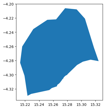
We are interested in the area of the capital city of Congo, Brazzaville. We therefore clip the road network to the shapefile of the city
# This is the GeoPandas dataframe
display(city)
city.plot()
| ID_0 | COUNTRY | NAME_1 | NL_NAME_1 | ID_2 | NAME_2 | VARNAME_2 | NL_NAME_2 | TYPE_2 | ENGTYPE_2 | CC_2 | HASC_2 | geometry | |
|---|---|---|---|---|---|---|---|---|---|---|---|---|---|
| 0 | COG | Republic of the Congo | Brazzaville | NaN | COG.2.1_1 | Brazzaville | NaN | NaN | District | District | NaN | CG.BR.BR | POLYGON ((15.32458 -4.28091, 15.31317 -4.27887... |
<Axes: >
# This is the Shapely geometry object contained in the geodf
city_shp = city.geometry[0]
city_shp

We check to see everything lines up by running intersect and counting the True / False returns. The count of the True values are the number of roads that intersect the AOI
intersects is a Shapely function that returns True if the boundary or interior of the object intersect in any way with those of the other
roads_osm.roads_raw.to_crs(epsg)
print(roads_osm.roads_raw.crs)
print(city.crs)
+init=epsg:4326 +type=crs
EPSG:4326
roads_osm.roads_raw.geometry.intersects(city_shp).value_counts()
False    48701
True      5986
Name: count, dtype: int64
We can therefore remove any roads that does not intersect Brazzaville administrative unit
roads_osm.roads_raw = roads_osm.roads_raw.loc[roads_osm.roads_raw.geometry.intersects(city_shp) == True]
Now we generate the RoadsGPD object, which is stored as a property of the ‘OSM_to_network’ object. The RoadsGPD object is a GeoDataFrame that further processes the roads.
This includes splitting the edges where intersections occur, adding unique edge IDs, and adding to/from columns to the GeoDataFrame.
We can do this using the generateRoadsGDF function
roads_osm.generateRoadsGDF(verbose = False)
We use the initialReadIn() function to transform this to a graph object
roads_osm.initialReadIn()
<networkx.classes.multidigraph.MultiDiGraph at 0x729fa47b36a0>
?roads_osm.network
Type:           MultiDiGraph
String form:    MultiDiGraph with 14031 nodes and 21554 edges
Length:         14031
File:           ~/.conda/envs/geo_wb_linux/lib/python3.8/site-packages/networkx/classes/multidigraph.py
Docstring:
A directed graph class that can store multiedges.

Multiedges are multiple edges between two nodes.  Each edge
can hold optional data or attributes.

A MultiDiGraph holds directed edges.  Self loops are allowed.

Nodes can be arbitrary (hashable) Python objects with optional
key/value attributes. By convention `None` is not used as a node.

Edges are represented as links between nodes with optional
key/value attributes.

Parameters
----------
incoming_graph_data : input graph (optional, default: None)
    Data to initialize graph. If None (default) an empty
    graph is created.  The data can be any format that is supported
    by the to_networkx_graph() function, currently including edge list,
    dict of dicts, dict of lists, NetworkX graph, 2D NumPy array, SciPy
    sparse matrix, or PyGraphviz graph.

multigraph_input : bool or None (default None)
    Note: Only used when `incoming_graph_data` is a dict.
    If True, `incoming_graph_data` is assumed to be a
    dict-of-dict-of-dict-of-dict structure keyed by
    node to neighbor to edge keys to edge data for multi-edges.
    A NetworkXError is raised if this is not the case.
    If False, :func:`to_networkx_graph` is used to try to determine
    the dict's graph data structure as either a dict-of-dict-of-dict
    keyed by node to neighbor to edge data, or a dict-of-iterable
    keyed by node to neighbors.
    If None, the treatment for True is tried, but if it fails,
    the treatment for False is tried.

attr : keyword arguments, optional (default= no attributes)
    Attributes to add to graph as key=value pairs.

See Also
--------
Graph
DiGraph
MultiGraph

Examples
--------
Create an empty graph structure (a "null graph") with no nodes and
no edges.

>>> G = nx.MultiDiGraph()

G can be grown in several ways.

**Nodes:**

Add one node at a time:

>>> G.add_node(1)

Add the nodes from any container (a list, dict, set or
even the lines from a file or the nodes from another graph).

>>> G.add_nodes_from([2, 3])
>>> G.add_nodes_from(range(100, 110))
>>> H = nx.path_graph(10)
>>> G.add_nodes_from(H)

In addition to strings and integers any hashable Python object
(except None) can represent a node, e.g. a customized node object,
or even another Graph.

>>> G.add_node(H)

**Edges:**

G can also be grown by adding edges.

Add one edge,

>>> key = G.add_edge(1, 2)

a list of edges,

>>> keys = G.add_edges_from([(1, 2), (1, 3)])

or a collection of edges,

>>> keys = G.add_edges_from(H.edges)

If some edges connect nodes not yet in the graph, the nodes
are added automatically.  If an edge already exists, an additional
edge is created and stored using a key to identify the edge.
By default the key is the lowest unused integer.

>>> keys = G.add_edges_from([(4, 5, dict(route=282)), (4, 5, dict(route=37))])
>>> G[4]
AdjacencyView({5: {0: {}, 1: {'route': 282}, 2: {'route': 37}}})

**Attributes:**

Each graph, node, and edge can hold key/value attribute pairs
in an associated attribute dictionary (the keys must be hashable).
By default these are empty, but can be added or changed using
add_edge, add_node or direct manipulation of the attribute
dictionaries named graph, node and edge respectively.

>>> G = nx.MultiDiGraph(day="Friday")
>>> G.graph
{'day': 'Friday'}

Add node attributes using add_node(), add_nodes_from() or G.nodes

>>> G.add_node(1, time="5pm")
>>> G.add_nodes_from([3], time="2pm")
>>> G.nodes[1]
{'time': '5pm'}
>>> G.nodes[1]["room"] = 714
>>> del G.nodes[1]["room"]  # remove attribute
>>> list(G.nodes(data=True))
[(1, {'time': '5pm'}), (3, {'time': '2pm'})]

Add edge attributes using add_edge(), add_edges_from(), subscript
notation, or G.edges.

>>> key = G.add_edge(1, 2, weight=4.7)
>>> keys = G.add_edges_from([(3, 4), (4, 5)], color="red")
>>> keys = G.add_edges_from([(1, 2, {"color": "blue"}), (2, 3, {"weight": 8})])
>>> G[1][2][0]["weight"] = 4.7
>>> G.edges[1, 2, 0]["weight"] = 4

Warning: we protect the graph data structure by making `G.edges[1,
2, 0]` a read-only dict-like structure. However, you can assign to
attributes in e.g. `G.edges[1, 2, 0]`. Thus, use 2 sets of brackets
to add/change data attributes: `G.edges[1, 2, 0]['weight'] = 4`
(for multigraphs the edge key is required: `MG.edges[u, v,
key][name] = value`).

**Shortcuts:**

Many common graph features allow python syntax to speed reporting.

>>> 1 in G  # check if node in graph
True
>>> [n for n in G if n < 3]  # iterate through nodes
[1, 2]
>>> len(G)  # number of nodes in graph
5
>>> G[1]  # adjacency dict-like view mapping neighbor -> edge key -> edge attributes
AdjacencyView({2: {0: {'weight': 4}, 1: {'color': 'blue'}}})

Often the best way to traverse all edges of a graph is via the neighbors.
The neighbors are available as an adjacency-view `G.adj` object or via
the method `G.adjacency()`.

>>> for n, nbrsdict in G.adjacency():
...     for nbr, keydict in nbrsdict.items():
...         for key, eattr in keydict.items():
...             if "weight" in eattr:
...                 # Do something useful with the edges
...                 pass

But the edges() method is often more convenient:

>>> for u, v, keys, weight in G.edges(data="weight", keys=True):
...     if weight is not None:
...         # Do something useful with the edges
...         pass

**Reporting:**

Simple graph information is obtained using methods and object-attributes.
Reporting usually provides views instead of containers to reduce memory
usage. The views update as the graph is updated similarly to dict-views.
The objects `nodes`, `edges` and `adj` provide access to data attributes
via lookup (e.g. `nodes[n]`, `edges[u, v, k]`, `adj[u][v]`) and iteration
(e.g. `nodes.items()`, `nodes.data('color')`,
`nodes.data('color', default='blue')` and similarly for `edges`)
Views exist for `nodes`, `edges`, `neighbors()`/`adj` and `degree`.

For details on these and other miscellaneous methods, see below.

**Subclasses (Advanced):**

The MultiDiGraph class uses a dict-of-dict-of-dict-of-dict structure.
The outer dict (node_dict) holds adjacency information keyed by node.
The next dict (adjlist_dict) represents the adjacency information
and holds edge_key dicts keyed by neighbor. The edge_key dict holds
each edge_attr dict keyed by edge key. The inner dict
(edge_attr_dict) represents the edge data and holds edge attribute
values keyed by attribute names.

Each of these four dicts in the dict-of-dict-of-dict-of-dict
structure can be replaced by a user defined dict-like object.
In general, the dict-like features should be maintained but
extra features can be added. To replace one of the dicts create
a new graph class by changing the class(!) variable holding the
factory for that dict-like structure. The variable names are
node_dict_factory, node_attr_dict_factory, adjlist_inner_dict_factory,
adjlist_outer_dict_factory, edge_key_dict_factory, edge_attr_dict_factory
and graph_attr_dict_factory.

node_dict_factory : function, (default: dict)
    Factory function to be used to create the dict containing node
    attributes, keyed by node id.
    It should require no arguments and return a dict-like object

node_attr_dict_factory: function, (default: dict)
    Factory function to be used to create the node attribute
    dict which holds attribute values keyed by attribute name.
    It should require no arguments and return a dict-like object

adjlist_outer_dict_factory : function, (default: dict)
    Factory function to be used to create the outer-most dict
    in the data structure that holds adjacency info keyed by node.
    It should require no arguments and return a dict-like object.

adjlist_inner_dict_factory : function, (default: dict)
    Factory function to be used to create the adjacency list
    dict which holds multiedge key dicts keyed by neighbor.
    It should require no arguments and return a dict-like object.

edge_key_dict_factory : function, (default: dict)
    Factory function to be used to create the edge key dict
    which holds edge data keyed by edge key.
    It should require no arguments and return a dict-like object.

edge_attr_dict_factory : function, (default: dict)
    Factory function to be used to create the edge attribute
    dict which holds attribute values keyed by attribute name.
    It should require no arguments and return a dict-like object.

graph_attr_dict_factory : function, (default: dict)
    Factory function to be used to create the graph attribute
    dict which holds attribute values keyed by attribute name.
    It should require no arguments and return a dict-like object.

Typically, if your extension doesn't impact the data structure all
methods will inherited without issue except: `to_directed/to_undirected`.
By default these methods create a DiGraph/Graph class and you probably
want them to create your extension of a DiGraph/Graph. To facilitate
this we define two class variables that you can set in your subclass.

to_directed_class : callable, (default: DiGraph or MultiDiGraph)
    Class to create a new graph structure in the `to_directed` method.
    If `None`, a NetworkX class (DiGraph or MultiDiGraph) is used.

to_undirected_class : callable, (default: Graph or MultiGraph)
    Class to create a new graph structure in the `to_undirected` method.
    If `None`, a NetworkX class (Graph or MultiGraph) is used.

**Subclassing Example**

Create a low memory graph class that effectively disallows edge
attributes by using a single attribute dict for all edges.
This reduces the memory used, but you lose edge attributes.

>>> class ThinGraph(nx.Graph):
...     all_edge_dict = {"weight": 1}
...
...     def single_edge_dict(self):
...         return self.all_edge_dict
...
...     edge_attr_dict_factory = single_edge_dict
>>> G = ThinGraph()
>>> G.add_edge(2, 1)
>>> G[2][1]
{'weight': 1}
>>> G.add_edge(2, 2)
>>> G[2][1] is G[2][2]
True
Init docstring:
Initialize a graph with edges, name, or graph attributes.

Parameters
----------
incoming_graph_data : input graph
    Data to initialize graph.  If incoming_graph_data=None (default)
    an empty graph is created.  The data can be an edge list, or any
    NetworkX graph object.  If the corresponding optional Python
    packages are installed the data can also be a 2D NumPy array, a
    SciPy sparse array, or a PyGraphviz graph.

multigraph_input : bool or None (default None)
    Note: Only used when `incoming_graph_data` is a dict.
    If True, `incoming_graph_data` is assumed to be a
    dict-of-dict-of-dict-of-dict structure keyed by
    node to neighbor to edge keys to edge data for multi-edges.
    A NetworkXError is raised if this is not the case.
    If False, :func:`to_networkx_graph` is used to try to determine
    the dict's graph data structure as either a dict-of-dict-of-dict
    keyed by node to neighbor to edge data, or a dict-of-iterable
    keyed by node to neighbors.
    If None, the treatment for True is tried, but if it fails,
    the treatment for False is tried.

attr : keyword arguments, optional (default= no attributes)
    Attributes to add to graph as key=value pairs.

See Also
--------
convert

Examples
--------
>>> G = nx.Graph()  # or DiGraph, MultiGraph, MultiDiGraph, etc
>>> G = nx.Graph(name="my graph")
>>> e = [(1, 2), (2, 3), (3, 4)]  # list of edges
>>> G = nx.Graph(e)

Arbitrary graph attribute pairs (key=value) may be assigned

>>> G = nx.Graph(e, day="Friday")
>>> G.graph
{'day': 'Friday'}
We save this graph object down to file using gn.save().
The save function produces three outputs: a node GeoDataFrame as a CSV, an edge GeoDataFrame as a CSV, and a graph object saved as a pickle (check your folder!).
gn.save(roads_osm.network,'roads_brazzaville',out_path)
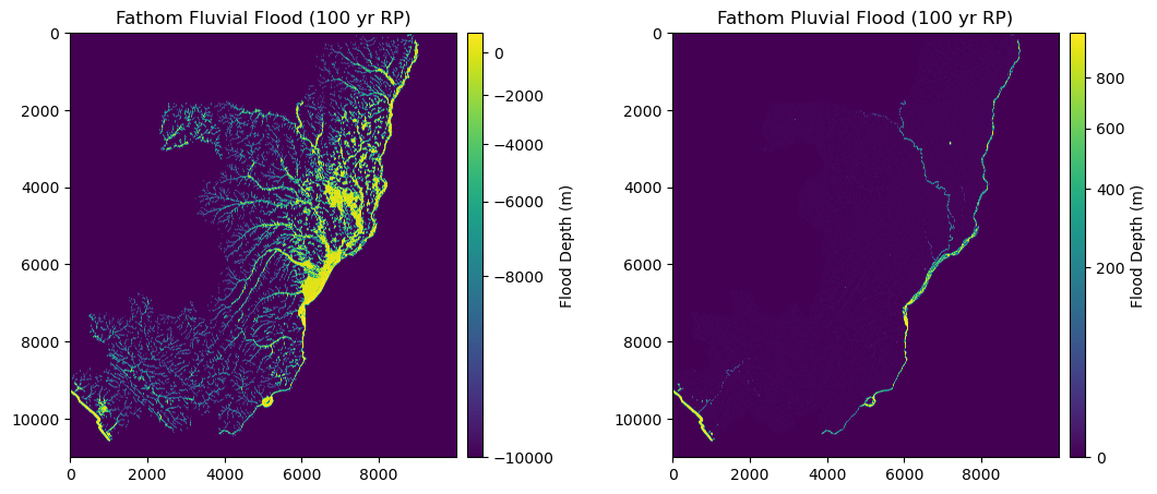
Import Flood extent and depth (.tif)#
Here, we import Fathom v2 Pluvial and Fluvial flood data (.tif) of 100 yr return period.
This represents and mimics one of the impacts that climate has on infrastructure and the disruption of the accessibility to health facilities.
flood_fluvial = rio.open(join(data_dir,"FU_1in100.tif")) #.read(1)
flood_pluvial = rio.open(join(data_dir,"P_1in100.tif")) #.read(1)
We can check the metadata, resolution and extent of the raster (in degrees)
meta = flood_pluvial.meta
meta
{'driver': 'GTiff',
 'dtype': 'float32',
 'nodata': None,
 'width': 10000,
 'height': 11000,
 'count': 1,
 'crs': CRS.from_epsg(4326),
 'transform': Affine(0.0008333333333333334, 0.0, 11.157916666668333,
        0.0, -0.0008333333333333334, 3.7495833336863327)}
flood_pluvial.bounds
BoundingBox(left=11.157916666668333, bottom=-5.417083332980335, right=19.491250000001667, top=3.7495833336863327)
flood_pluvial.res
(0.0008333333333333334, 0.0008333333333333334)
Rasterio datasets generally have one or more bands (e.g. EO images).
Following the GDAL convention, these bands are indexed starting with the number 1 (we have just 1 band in this case)
We import the file with the open() and read() function as a numpy.array
flood_fluvial = flood_fluvial.read(1)
flood_pluvial = flood_pluvial.read(1)
flood_fluvial
array([[-9999., -9999., -9999., ..., -9999., -9999., -9999.],
       [-9999., -9999., -9999., ..., -9999., -9999., -9999.],
       [-9999., -9999., -9999., ..., -9999., -9999., -9999.],
       ...,
       [-9999., -9999., -9999., ..., -9999., -9999., -9999.],
       [-9999., -9999., -9999., ..., -9999., -9999., -9999.],
       [-9999., -9999., -9999., ..., -9999., -9999., -9999.]],
      dtype=float32)
The two datasets have different missing values:
FLUVIAL:
not-flooded areas = -9999
inland water bodies and ocean = 999PLUVIAL:
not-flooded areas = 0
inland water bodies and ocean = 999
fig = plt.figure(figsize=(12, 8))  # Increase width to accommodate two panels
grid = fig.add_gridspec(1, 3, width_ratios=[1, 0.05, 1], wspace=0.3)  # Create grid layout

# First panel
ax1 = fig.add_subplot(grid[0, 0])
ax1.set_title("Fathom Fluvial Flood (100 yr RP)", fontsize=12, horizontalalignment='center')
im1 = ax1.imshow(flood_fluvial, norm=colors.PowerNorm(gamma=0.5), cmap='viridis')
divider1 = make_axes_locatable(ax1)
cax1 = divider1.append_axes('right', size="4%", pad=0.1)
cb1 = fig.colorbar(im1, cax=cax1, orientation='vertical')
cb1.set_label("Flood Depth (m)")

# Second panel
ax2 = fig.add_subplot(grid[0, 2])
ax2.set_title("Fathom Pluvial Flood (100 yr RP)", fontsize=12, horizontalalignment='center')
im2 = ax2.imshow(flood_pluvial, norm=colors.PowerNorm(gamma=0.5), cmap='viridis')
divider2 = make_axes_locatable(ax2)
cax2 = divider2.append_axes('right', size="4%", pad=0.1)
cb2 = fig.colorbar(im2, cax=cax2, orientation='vertical')
cb2.set_label("Flood Depth (m)")

plt.show()
We want to consider both the scenarios, therefore we preserve, among the two, the maximum flood depth
flood = np.fmax(flood_fluvial, flood_pluvial)
We can export and save the combined Flood dataset as a .tif file
with rio.open(join(data_dir,"Fmax_1in100.tif"), 'w', **meta) as dst:
            dst.write(flood, 1)
flood = rio.open(join(data_dir,"Fmax_1in100.tif"))
For the moment, we are only interested in Brazaville city, therefore we clip our raster with the city shapefile.
We can accomplish that by using the clipRaster function of GOSTrock library:
rMisc.clipRaster(flood, city, join(data_dir,"Fmax_1in100_clip.tif"), crop=True)
flood = rio.open(join(data_dir,"Fmax_1in100_clip.tif"))
For simplicity, we just substitute the value for open waters (999) to 0
flood_data = flood.read(1)
flood_data[flood_data == 999] = 0
Import the Health Facilities (destinations)#
Health facilities are stored as Geopandas dataframe
hf = gpd.read_file((data_dir+"/hf_COG.shp"))
hf = hf[hf.geometry.intersects(city_shp)]
display('The following categories and numbers of Health Facilities are considered to perform the analysis: ')
display(hf["Facility t"].value_counts())
'The following categories and numbers of Health Facilities are considered to perform the analysis: '
Facility t
Centre de Santé Intégré    22
l?Hôpital de Base           2
University Hospital         1
Name: count, dtype: int64
Import Population (origin)#
# wp_path = join(expanduser("R:/"), 'Data', 'GLOBAL/Population/WorldPop_PPP_2020/MOSAIC_ppp_prj_2020', f'ppp_prj_2020_{iso}.tif') # Download from link above
wp_path = join(data_dir, f'ppp_2020_1km_Aggregated.tif') # Download from link above

pop_surf = rio.open(wp_path)
pop_surf.res
(0.0083333333, 0.0083333333)
Health Facilities flood disruption#
Health facilities impacted by floods are identified. Similarly to the roads, when water level is >20 cm, the HF is considered as disrupted.
coords = [(x,y) for x, y in zip(hf.geometry.x, hf.geometry.y)]
hf["Flood_100"] = [x[0] for x in flood.sample(coords)]
hf_flooded = hf[hf["Flood_100"] > 0.2]
hf_dry = hf[~hf.index.isin(hf_flooded.index)]
Road network flood disruption#
Floods can impact all the roads, except the bridges in primary and secondary roads
flood_road = flood.read(1).copy()
safe_crit = ((roads_osm.roads_raw['bridge'] == "True") & ((roads_osm.roads_raw['infra_type'] == "primary") | (roads_osm.roads_raw['infra_type'] == "secondary")))
roads_safe = roads_osm.roads_raw[safe_crit]
roads_flood = roads_osm.roads_raw[~safe_crit]
Subsequently, we consider that if water level is more than 20 cm, the road is disrupted.
Therefore we mask our flood raster dataset, retaining only those pixels for which the flood depth is > 0.2 m
transf = flood.transform
mask = (flood_road >= 0.2)
Now, we have the roads stored as VECTORS (geodf) and the flood surface as RASTER (numpy).
To disrupt the roads network, we need to intersect the two datasets.
To do that, one option is to transform the flood raster into a vector polygon
# Create Polygons only from those cells where mask = True (water level >= 20 cm)
def raster_cells_to_polygons(mask, transform):

    polygons = []
    for (row, col), value in np.ndenumerate(mask):
            if value:         # Only create polygons where the mask is True
                # Get the coordinates of the top left corner of the cell
                top_left = rio.transform.xy(transform, row, col, offset='ul')
                # Since each cell is a square, calculate the bottom right corner
                bottom_right = rio.transform.xy(transform, row+1, col+1, offset='ul')
                # Create a polygon from these coordinates
                polygon = box(top_left[0], bottom_right[1], bottom_right[0], top_left[1])
                polygons.append(polygon)

    return polygons
# Vectorize the masked cells
flood_poly = raster_cells_to_polygons(mask, transf)
flood_poly_gdf = gpd.GeoDataFrame(geometry=flood_poly, crs=epsg)  # Make sure to set the correct CRS
flood_poly_gdf
| geometry | |
|---|---|
| 0 | POLYGON ((15.28792 -4.21208, 15.28792 -4.21125... |
| 1 | POLYGON ((15.28792 -4.21292, 15.28792 -4.21208... |
| 2 | POLYGON ((15.28875 -4.21292, 15.28875 -4.21208... |
| 3 | POLYGON ((15.29792 -4.21292, 15.29792 -4.21208... |
| 4 | POLYGON ((15.29875 -4.21292, 15.29875 -4.21208... |
| ... | ... |
| 4005 | POLYGON ((15.22458 -4.32958, 15.22458 -4.32875... |
| 4006 | POLYGON ((15.22542 -4.32958, 15.22542 -4.32875... |
| 4007 | POLYGON ((15.22625 -4.32958, 15.22625 -4.32875... |
| 4008 | POLYGON ((15.22375 -4.33042, 15.22375 -4.32958... |
| 4009 | POLYGON ((15.22458 -4.33042, 15.22458 -4.32958... |
4010 rows × 1 columns
Now that our flood dataset is a GeoPandas DataFrame, we can compute the intersection with the road network
intersect = gpd.sjoin(roads_flood, flood_poly_gdf, how="inner", op='intersects')
We remove the duplicates, since one road could be intersected by multiple flooded cells, and thus appear multiple times in the results
intersect.drop_duplicates(subset="osm_id", inplace = True)
intersect
| osm_id | infra_type | one_way | bridge | geometry | index_right | |
|---|---|---|---|---|---|---|
| 3 | 4692231 | primary | True | False | LINESTRING (15.28165 -4.27427, 15.28176 -4.274... | 1670 |
| 5 | 4692249 | primary | True | False | LINESTRING (15.26843 -4.28297, 15.26847 -4.282... | 1670 |
| 27 | 23342339 | residential | False | False | LINESTRING (15.27811 -4.27821, 15.27909 -4.277... | 1670 |
| 244 | 37363116 | unclassified | False | False | LINESTRING (15.28150 -4.27443, 15.28160 -4.274... | 1670 |
| 26845 | 422471832 | primary | True | False | LINESTRING (15.28163 -4.27433, 15.28165 -4.274... | 1670 |
| ... | ... | ... | ... | ... | ... | ... |
| 48823 | 775215093 | path | False | True | LINESTRING (15.24864 -4.27662, 15.24864 -4.276... | 1901 |
| 48800 | 773158924 | path | False | True | LINESTRING (15.24610 -4.27926, 15.24599 -4.279... | 1953 |
| 54201 | 1222996295 | service | False | False | LINESTRING (15.29389 -4.27222, 15.29371 -4.272... | 1583 |
| 54202 | 1222996296 | footway | False | False | LINESTRING (15.29378 -4.27264, 15.29369 -4.272... | 1583 |
| 54203 | 1222996297 | footway | False | False | LINESTRING (15.29389 -4.27222, 15.29395 -4.272... | 1584 |
977 rows × 6 columns
Finally, we remove the roads that are flooded (intersect) by matching their index, and modify the road network merging the “safe” roads with the disrupted.
roads_impact = roads_osm.roads_raw.drop(intersect.index)
roads_osm.roads_raw = pd.concat([roads_impact, roads_safe], axis = 0)
We apply the following commands again, to update the graph object considering the flooding scenario:
roads_osm.generateRoadsGDF(verbose = False)
roads_osm.initialReadIn()
We save the graph object of the flooded roads down to file using gn.save().
gn.save(roads_osm.network,'roads_brazzaville_flooded',out_path)
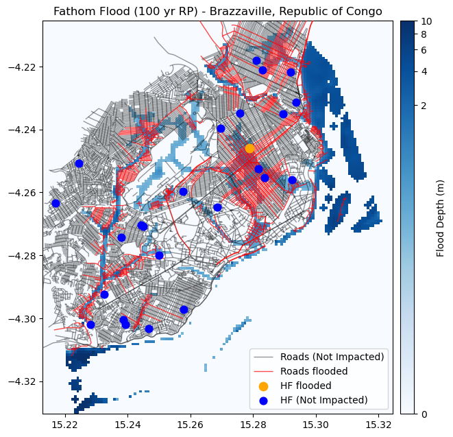
Let’s plot the location of the Health facilities, together with the flood dataset and the roads
fig, ax = plt.subplots(figsize=(7, 8))
ax.set_title("Fathom Flood (100 yr RP) - Brazzaville, Republic of Congo", fontsize=12, horizontalalignment='center')

# Plot the flood data
flood_image = show(flood_data, transform=flood.transform, ax=ax, norm=colors.PowerNorm(gamma=0.15), cmap='Blues', alpha = 1, zorder = 2)

# Create an axis divider for the colorbar
divider = make_axes_locatable(ax)
cax = divider.append_axes('right', size="4%", pad=0.1)

# Add the colorbar
cb = fig.colorbar(flood_image.get_images()[0], cax=cax, orientation='vertical')
cb.set_label("Flood Depth (m)")

# Plot the road network not impcted
roads_osm.roads_raw.plot(ax=ax, color='black', linewidth=1, alpha = 0.4, zorder = 2, label='Roads (Not Impacted)')
# Plot the road network disrupted
intersect.plot(ax=ax, color='red', linewidth=1, alpha = 0.7, zorder = 3, label='Roads flooded')
# PLot the Health facilities flooded
hf_flooded.plot(ax=ax, color='orange', markersize = 80, zorder=3, label='HF flooded')
# Plot the Health facilities not affected
hf_dry.plot(ax=ax, color='blue', markersize = 60, zorder=3, label='HF (Not Impacted)')

ax.set_xlim(flood.bounds.left, flood.bounds.right)
ax.set_ylim(flood.bounds.bottom, flood.bounds.top)

ax.legend(loc='lower right')

plt.show()
Calculate Betweeness centrality#
with open(os.path.join(out_path, 'roads_brazzaville.gpickle'), 'rb') as f:
    G = pickle.load(f)

with open(os.path.join(out_path, 'roads_brazzaville_flooded.gpickle'), 'rb') as f:
    G_flood = pickle.load(f)
print(G)
print(G_flood)
MultiDiGraph with 14031 nodes and 21554 edges
MultiDiGraph with 10966 nodes and 15687 edges
def create_grid(bbox, x_distance, y_distance):
    x = np.arange(bbox[0], bbox[2], x_distance)
    y = np.arange(bbox[1], bbox[3], y_distance)
    Y, X = np.meshgrid(y, x, indexing="ij")
    #create a iterable with the (x,y) coordinates
    points = [Point(x,y) for x, y in zip(X.flatten(),Y.flatten())]
    points_raw = [(x,y) for x, y in zip(X.flatten(),Y.flatten())]
    return gpd.GeoDataFrame(geometry=points, crs=4326)
start_points = create_grid(flood.bounds, 0.01, 0.01)
start_points
---------------------------------------------------------------------------
NameError                                 Traceback (most recent call last)
Cell In[1], line 1
----> 1 start_points

NameError: name 'start_points' is not defined
G_clean = gn.clean_network(G, UTM = epsg_utm, WGS = epsg, junctdist = 10, verbose = False)
G_flood_clean = gn.clean_network(G_flood, UTM = epsg_utm, WGS = epsg, junctdist = 10, verbose = False)
21554
completed processing 43108 edges
20985
completed processing 41970 edges
Edge reduction: 21554 to 41970 (-94 percent)
15687
completed processing 31374 edges
15205
completed processing 30410 edges
Edge reduction: 15687 to 30410 (-93 percent)
G.graph['crs'] = epsg
G_flood.graph['crs'] = epsg
Calculate the betweeeness centrality under both normal and flooded conditions.
find the shortest path from the origin (point on grid) to the destination (HF)
retrieve all the edges along the shortest path
count the number of times an edge is part of a shortest path
%%time

routes = []
for i, h in hf.iterrows():
   for i, s in start_points.iterrows():
        orig = ox.nearest_nodes(G, Y=s.geometry.y, X=s.geometry.x)
        dest = ox.nearest_nodes(G, Y=h.geometry.y, X=h.geometry.x)
        try:
            route = nx.shortest_path(G, orig, dest, weight="travel_time")
        except Exception as e:
            #print(e)
            continue
        try:
            route_df = ox.utils_graph.route_to_gdf(G, route, weight='length').reset_index()
        except ValueError as e:
            #print(e)
            continue
        routes.append(route_df)
CPU times: user 8min 56s, sys: 6.37 s, total: 9min 2s
Wall time: 9min 1s
%%time

routes_flood = []
for i, h in hf_dry.iterrows():
    for i, s in start_points.iterrows():
        orig = ox.nearest_nodes(G_flood, Y=s.geometry.y, X=s.geometry.x)
        dest = ox.nearest_nodes(G_flood, Y=h.geometry.y, X=h.geometry.x)
        try:
            route = nx.shortest_path(G_flood, orig, dest, weight="travel_time")
        except Exception as e:
            #print(e)
            continue
        try:
            route_df = ox.utils_graph.route_to_gdf(G_flood, route, weight='length').reset_index()
        except ValueError as e:
            #print(e)
            continue
        routes_flood.append(route_df)
CPU times: user 6min 10s, sys: 4.52 s, total: 6min 14s
Wall time: 6min 14s
routes_df = pd.concat(routes)
routes_df_flood = pd.concat(routes_flood)
# Here, after applying the count() function, we could take every variable, not uniquely "length", as they represent the result of the counter
route_count = routes_df.groupby(['u', 'v', 'key']).count()['length']; route_count.name = 'route_count'
route_count_flood = routes_df_flood.groupby(['u', 'v', 'key']).count()['length']; route_count_flood.name = 'route_count_flood'
nodes_df, edges_df = ox.graph_to_gdfs(G)
edges_df = edges_df.join(route_count)
edges_df['centrality'] = edges_df['route_count'] / edges_df['route_count'].max()

nodes_df_flood, edges_df_flood = ox.graph_to_gdfs(G_flood)
edges_df_flood = edges_df_flood.join(route_count_flood)
edges_df_flood['centrality'] = edges_df_flood['route_count_flood'] / edges_df_flood['route_count_flood'].max()
fig, ax = plt.subplots(figsize=(6, 8))
ax.set_title("Betweenness centrality - Brazzaville, Republic of Congo", fontsize=12, horizontalalignment='center')

# Plot the flood data
flood_image = show(flood_data, transform=flood.transform, ax=ax, norm=colors.PowerNorm(gamma=0.15), cmap='Blues', alpha = 1, zorder = 2)

# Create an axis divider for the colorbar
divider = make_axes_locatable(ax)
cax = divider.append_axes('right', size="4%", pad=0.1)

# Add the colorbar
cb = fig.colorbar(flood_image.get_images()[0], cax=cax, orientation='vertical')
cb.set_label("Flood Depth (m)")

# Plot the road network impcted
edges_df_flood.plot(ax = ax, column='centrality',  cmap='magma_r', zorder = 3)

# PLot the Health facilities flooded
hf_flooded.plot(ax=ax, color='orange', markersize = 80, zorder=3, label='HF flooded')
# Plot the Health facilities not affected
hf_dry.plot(ax=ax, color='blue', markersize = 60, zorder=3, label='HF (Not Impacted)')

ax.set_xlim(flood.bounds.left, flood.bounds.right)
ax.set_ylim(flood.bounds.bottom, flood.bounds.top)

plt.show()
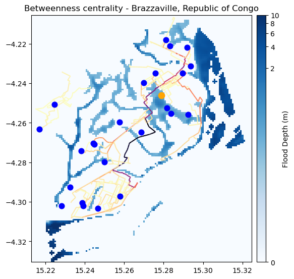
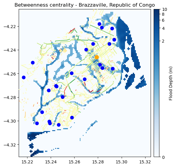
If the centrality is reduced, the road is not a good backup one, indicating potential lack of resilience on that pathway.
If the centrality is increased, on the other hand, that segment is a good backup road, and deserves attention during disasters and potential investments
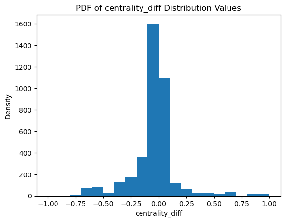
# Merge the dataframes on "osm_id"
centrality_diff = edges_df_flood.merge(edges_df, on="id", suffixes=('_flood', ''))
# Replace NaN with 0
centrality_diff["centrality_flood"].fillna(0, inplace=True)
centrality_diff["centrality"].fillna(0, inplace=True)

# Calculate the centrality difference
centrality_diff["centrality_diff"] = centrality_diff["centrality_flood"] - centrality_diff["centrality"]
centrality_diff["centrality_diff"].replace(0, np.nan, inplace=True)

# centrality_diff

plt.hist(centrality_diff["centrality_diff"], bins = 20)
plt.title('PDF of centrality_diff Distribution Values')
plt.xlabel('centrality_diff')
plt.ylabel('Density')
plt.show()
fig, ax = plt.subplots(figsize=(6, 8))
ax.set_title("Betweenness centrality - Brazzaville, Republic of Congo", fontsize=12, horizontalalignment='center')

# Plot the flood data
flood_image = show(flood_data, transform=flood.transform, ax=ax, norm=colors.PowerNorm(gamma=0.15), cmap='Blues', alpha = 1, zorder = 2)

# Create an axis divider for the colorbar
divider = make_axes_locatable(ax)
cax = divider.append_axes('right', size="4%", pad=0.1)

# Add the colorbar
cb = fig.colorbar(flood_image.get_images()[0], cax=cax, orientation='vertical')
cb.set_label("Flood Depth (m)")

# Plot the road network impacted
centrality_diff.plot(ax = ax, column='centrality_diff',  cmap='RdYlGn_r', zorder = 3)

# PLot the Health facilities flooded
hf_flooded.plot(ax=ax, color='orange', markersize = 80, zorder=3, label='HF flooded')
# Plot the Health facilities not affected
hf_dry.plot(ax=ax, color='blue', markersize = 60, zorder=3, label='HF (Not Impacted)')

ax.set_xlim(flood.bounds.left, flood.bounds.right)
ax.set_ylim(flood.bounds.bottom, flood.bounds.top)

# ax.legend(loc='lower right')

plt.show()