Tutorial - Module 2: Accessibility Analysis

This notebook is a template workflow to collect data and prepare the main data to perform a baseline physical accessibility analysis to health facilities. It uses various tools developed by the World Bank’s Geospatial Operations Support Team (GOST).

This notebook represents the second module of the tutorial on the physical accessibility to health facilities in a context of emergency.
It focuses on the datasets and the functions to be used to perform the analysis. A particular focus will be put on the uncertainty and pros&cons deriving from the utilization of different datasets. \

Setup

Import packages required for the analysis

# System
import sys
import os
from os.path import join, expanduser
from pathlib import Path
# Avoid warnings to pop up
import warnings
warnings.filterwarnings('ignore')

# Visualization tools
# import folium as flm
import matplotlib.pyplot as plt
import matplotlib.colors as colors
import matplotlib.gridspec as gridspec
from rasterio.plot import plotting_extent
from rasterio.plot import show
from mpl_toolkits.axes_grid1 import make_axes_locatable
import contextily as ctx
import cartopy
import cartopy.crs as ccrs
import cartopy.feature as cfeature
import seaborn as sns

os.environ['CARTOPY_USER_BACKGROUNDS'] = '/home/jupyter-wb618081/Python/Backgrounds/'

# Processing 
import numpy as np
import geopandas as gpd
import pandas as pd
from gadm import GADMDownloader
import dask_geopandas as dask_gpd

# Raster
import rasterio as rio
from rasterio.features import shapes
from shapely.geometry import box
from rasterio.features import geometry_mask
from rasterstats import zonal_stats
from shapely.geometry import Polygon, box, Point
from shapely.geometry import mapping
import skimage.graph as graph
from scipy.signal import convolve2d

# Graph
import pickle
import networkx as nx
import osmnx as ox

# for facebook data
from pyquadkey2 import quadkey

# Climate/Flood
# import xarray as xr

# Define your path to the Repositories

sys.path.append(join(expanduser("/home/jupyter-wb618081"), 'Repos', 'gostrocks', 'src'))
sys.path.append(join(expanduser("/home/jupyter-wb618081"), 'Repos', 'GOSTNets_Raster', 'src'))
sys.path.append(join(expanduser("/home/jupyter-wb618081"), 'Repos', 'GOSTnets'))
sys.path.append(join(expanduser("/home/jupyter-wb618081"), 'Repos', 'GOST_Urban', 'src', 'GOST_Urban'))
sys.path.append(join(expanduser("/home/jupyter-wb618081"), 'Repos', 'health-equity-diagnostics', 'src', 'modules'))
sys.path.append(join(expanduser("/home/jupyter-wb618081"), 'Repos', 'INFRA_SAP'))

import GOSTnets as gn
from GOSTnets.load_osm import *
import GOSTRocks.rasterMisc as rMisc
from GOSTRocks.misc import get_utm
import GOSTNetsRaster.market_access as ma
import UrbanRaster as urban

from infrasap import aggregator
from infrasap import osm_extractor as osm   

from utils import download_osm_shapefiles

# auto reload
%load_ext autoreload
%autoreload 2

Define below the local folder where you are located

scratch_dir = join(expanduser("/home/jupyter-wb618081"), 'Health-Access-Metrics', 'Tutorials')
data_dir = join(scratch_dir, 'tutorial_data')
out_path = join(scratch_dir, 'tutorial_output')

## Function for creating a path, if needed ##
def checkDir(out_path):
    if not os.path.exists(out_path):
        os.makedirs(out_path)

Data Preparation

Import the City boundaries (.shp)

epsg = "EPSG:4326"
epsg_utm = "EPSG:28232"

country = 'Congo'
iso = 'COG'
city = gpd.read_file((data_dir+"/brazaville.shp"))
city.to_crs(epsg)
city

	ID_0	COUNTRY	NAME_1	NL_NAME_1	ID_2	NAME_2	VARNAME_2	NL_NAME_2	TYPE_2	ENGTYPE_2	CC_2	HASC_2	geometry
0	COG	Republic of the Congo	Brazzaville	NaN	COG.2.1_1	Brazzaville	NaN	NaN	District	District	NaN	CG.BR.BR	POLYGON ((15.32458 -4.28091, 15.31317 -4.27887...

Import the Road Network (.shp)

Download from the link above the OpenStreetMap road network from Geofabrik

roads_osm = OSM_to_network(join(data_dir,"congo-brazzaville-latest.osm.pbf"))

GOSTNets creates a special ‘OSM_to_network’ object. This object gets initialized with both a copy of the OSM file itself and the roads extracted from the OSM file in a GeoPandas DataFrame. This DataFrame is a property of the object called ‘roads_raw’ and is the starting point for our network.

?roads_osm

Type:           OSM_to_network
String form:    <GOSTnets.load_osm.OSM_to_network object at 0x7ec141828b20>
File:           ~/Repos/GOSTnets/GOSTnets/load_osm.py
Docstring:     
Object to load OSM PBF to networkX objects.

Object to load OSM PBF to networkX objects.     EXAMPLE:     G_loader = losm.OSM_to_network(bufferedOSM_pbf)     G_loader.generateRoadsGDF()     G = G.initialReadIn() 
snap origins and destinations     o_snapped = gn.pandana_snap(G, origins)     d_snapped = gn.pandana_snap(G, destinations)     
Init docstring: Generate a networkX object from a osm file

roads_gdf = roads_osm.roads_raw
roads_osm.roads_raw.head()

	osm_id	infra_type	one_way	bridge	geometry
0	4692113	primary	True	False	LINESTRING (15.23126 -4.29689, 15.23134 -4.296...
1	4692179	primary	True	False	LINESTRING (15.25202 -4.28510, 15.25210 -4.285...
2	4692181	primary	True	False	LINESTRING (15.24010 -4.29174, 15.23988 -4.291...
3	4692231	primary	True	False	LINESTRING (15.28165 -4.27427, 15.28176 -4.274...
4	4692245	primary	True	False	LINESTRING (15.25944 -4.28030, 15.25946 -4.280...

?roads_osm.roads_raw

Type:        GeoDataFrame
String form:
osm_id   infra_type  one_way  bridge  \
           0         4692113      primary     True   Fals <...>  -4.785...
           54721  LINESTRING (11.94277 -4.78254, 11.94306 -4.784...
           
           [54722 rows x 5 columns]
Length:      54722
File:        ~/.conda/envs/geo_wb_linux/lib/python3.8/site-packages/geopandas/geodataframe.py
Docstring:  
A GeoDataFrame object is a pandas.DataFrame that has a column
with geometry. In addition to the standard DataFrame constructor arguments,
GeoDataFrame also accepts the following keyword arguments:

Parameters
----------
crs : value (optional)
    Coordinate Reference System of the geometry objects. Can be anything accepted by
    :meth:`pyproj.CRS.from_user_input() <pyproj.crs.CRS.from_user_input>`,
    such as an authority string (eg "EPSG:4326") or a WKT string.
geometry : str or array (optional)
    If str, column to use as geometry. If array, will be set as 'geometry'
    column on GeoDataFrame.

Examples
--------
Constructing GeoDataFrame from a dictionary.

>>> from shapely.geometry import Point
>>> d = {'col1': ['name1', 'name2'], 'geometry': [Point(1, 2), Point(2, 1)]}
>>> gdf = geopandas.GeoDataFrame(d, crs="EPSG:4326")
>>> gdf
    col1                 geometry
0  name1  POINT (1.00000 2.00000)
1  name2  POINT (2.00000 1.00000)

Notice that the inferred dtype of 'geometry' columns is geometry.

>>> gdf.dtypes
col1          object
geometry    geometry
dtype: object

Constructing GeoDataFrame from a pandas DataFrame with a column of WKT geometries:

>>> import pandas as pd
>>> d = {'col1': ['name1', 'name2'], 'wkt': ['POINT (1 2)', 'POINT (2 1)']}
>>> df = pd.DataFrame(d)
>>> gs = geopandas.GeoSeries.from_wkt(df['wkt'])
>>> gdf = geopandas.GeoDataFrame(df, geometry=gs, crs="EPSG:4326")
>>> gdf
    col1          wkt                 geometry
0  name1  POINT (1 2)  POINT (1.00000 2.00000)
1  name2  POINT (2 1)  POINT (2.00000 1.00000)

See also
--------
GeoSeries : Series object designed to store shapely geometry objects

roads_osm.roads_raw.infra_type.value_counts()

infra_type
residential       35414
track              7667
unclassified       3599
path               2504
service            1696
tertiary           1608
trunk               746
secondary           655
primary             409
footway             297
primary_link         36
trunk_link           27
construction         21
tertiary_link        20
secondary_link        9
living_street         5
steps                 4
pedestrian            3
yes                   2
Name: count, dtype: int64

We can show the different highway types and counts

We need to define a list of the types of roads from the above that we consider acceptable for our road network

accepted_road_types = ['residential', 'track','unclassified','path', 'service','tertiary','trunk','secondary','primary',
                       'footway','primary_link','trunk_link','secondary_link','tertiary_link']

We can therefore filter our roads using the filterRoads method

roads_osm.filterRoads(acceptedRoads = accepted_road_types)

roads_osm.roads_raw.infra_type.value_counts()

infra_type
residential       35414
track              7667
unclassified       3599
path               2504
service            1696
tertiary           1608
trunk               746
secondary           655
primary             409
footway             297
primary_link         36
trunk_link           27
tertiary_link        20
secondary_link        9
Name: count, dtype: int64

We are interested in the area of the capital city of Congo, Brazzaville. We therefore clip the road network to the shapefile of the city

# This is the GeoPandas dataframe
display(city)
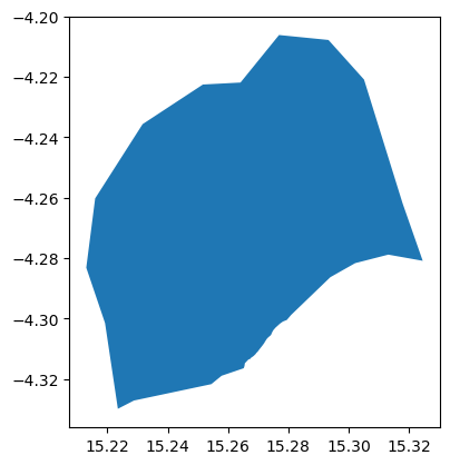
city.plot()

	ID_0	COUNTRY	NAME_1	NL_NAME_1	ID_2	NAME_2	VARNAME_2	NL_NAME_2	TYPE_2	ENGTYPE_2	CC_2	HASC_2	geometry
0	COG	Republic of the Congo	Brazzaville	NaN	COG.2.1_1	Brazzaville	NaN	NaN	District	District	NaN	CG.BR.BR	POLYGON ((15.32458 -4.28091, 15.31317 -4.27887...

<Axes: >

# This is the Shapely geometry object contained in the geodf
city_shp = city.geometry[0]
city_shp

We check to see everything lines up by running intersect and counting the True / False returns. The count of the True values are the number of roads that intersect the AOI
intersects is a Shapely function that returns True if the boundary or interior of the object intersect in any way with those of the other

roads_osm.roads_raw.to_crs(epsg)
print(roads_osm.roads_raw.crs)
print(city.crs)

+init=epsg:4326 +type=crs
EPSG:4326

roads_osm.roads_raw.geometry.intersects(city_shp).value_counts()

False    48701
True      5986
Name: count, dtype: int64

We can therefore remove any roads that does not intersect Brazzaville administrative unit

roads_osm.roads_raw = roads_osm.roads_raw.loc[roads_osm.roads_raw.geometry.intersects(city_shp) == True]

Now we generate the RoadsGPD object, which is stored as a property of the ‘OSM_to_network’ object. The RoadsGPD object is a GeoDataFrame that further processes the roads.
This includes splitting the edges where intersections occur, adding unique edge IDs, and adding to/from columns to the GeoDataFrame.
We can do this using the generateRoadsGDF function

roads_osm.generateRoadsGDF(verbose = False)

We use the initialReadIn() function to transform this to a graph object

roads_osm.initialReadIn()

<networkx.classes.multidigraph.MultiDiGraph at 0x7ebd20adefd0>

roads_osm.network

<networkx.classes.multidigraph.MultiDiGraph at 0x7ebd20adefd0>

We save this graph object down to file using gn.save().
The save function produces three outputs: a node GeoDataFrame as a CSV, an edge GeoDataFrame as a CSV, and a graph object saved as a pickle (check your folder!).

gn.save(roads_osm.network,'roads_brazzaville',out_path)

Import Friction Surface (.tif)

travel_surf = rio.open(join(data_dir, f"travel_surface_motorized_2020_{iso}.tif"))
travel_surf.res

(0.008333333333333333, 0.008333333333333333)

Import the Health Facilities (destinations)

Health facilities are stored as Geopandas dataframe

hf = gpd.read_file((data_dir+"/hf_COG.shp"))

hf = hf[hf.geometry.intersects(city_shp)]

display('The following categories and numbers of Health Facilities are considered to perform the analysis: ')
display(hf["Facility t"].value_counts())

'The following categories and numbers of Health Facilities are considered to perform the analysis: '

Facility t
Centre de Santé Intégré    22
l?Hôpital de Base           2
University Hospital         1
Name: count, dtype: int64

Import Population (origin)

# wp_path = join(expanduser("R:/"), 'Data', 'GLOBAL/Population/WorldPop_PPP_2020/MOSAIC_ppp_prj_2020', f'ppp_prj_2020_{iso}.tif') # Download from link above
wp_path = join(data_dir, f'cog_ppp_2020_1km_Aggregated.tif') # Download from link above
pop_surf = rio.open(wp_path)

rMisc.clipRaster(pop_surf, city, join(data_dir, f"pop_brazaville.tif"), crop=True)

wp_path = join(data_dir, f'pop_brazaville.tif')
pop_surf = rio.open(wp_path)

# Create a population df from population surface 
indices = list(np.ndindex(pop_surf.shape))
xys = [Point(pop_surf.xy(ind[0], ind[1])) for ind in indices]
res_df = pd.DataFrame({
    'spatial_index': indices,
    'geometry': xys,
    'pop': pop_surf.read(1).flatten()
})
res_df = res_df[res_df["pop"] != -99999.0]
res_df.head(2)

	spatial_index	geometry	pop
8	(0, 8)	POINT (15.277916606793564 -4.204583108029534)	7612.103027
9	(0, 9)	POINT (15.286249940093564 -4.204583108029534)	8549.582031

Let’s plot the location of the Health facilities, together with the travel surface dataset and the roads

fig, ax = plt.subplots(figsize=(6, 8))
ax.set_title("Brazzaville, Republic of Congo", fontsize=12, horizontalalignment='center')

# Plot the flood data
pop_image = show(marketsheds, transform=travel_surf.transform, ax=ax, norm=colors.PowerNorm(gamma=0.15), cmap='viridis', alpha = 1, zorder = 2)
# travel_surf.read(1)*1000/60
# Create an axis divider for the colorbar
divider = make_axes_locatable(ax)
cax = divider.append_axes('right', size="4%", pad=0.1)

# Add the colorbar
cb = fig.colorbar(pop_image.get_images()[0], cax=cax, orientation='vertical')
cb.set_label("Hours for 1km cell")

# Plot the road network not impcted
roads_osm.roads_raw.plot(ax=ax, color='black', linewidth=1, alpha = 0.4, zorder = 2)
# PLot the Health facilities
hf.plot(ax=ax, color='red', markersize = 60, zorder=3)
city.boundary.plot(ax=ax, color = "black", zorder=3, edgecolor="black")

ax.set_xlim(city_shp.bounds[0], city_shp.bounds[2])
ax.set_ylim(city_shp.bounds[1], city_shp.bounds[3])

plt.show()

Calculate Travel Time

with open(os.path.join(out_path, 'roads_brazzaville.gpickle'), 'rb') as f:
    G = pickle.load(f)

print('start: %s\n' % time.ctime())
G_clean = gn.clean_network(G, wpath = out_path, output_file_name = 'roads_brazzaville_clean', UTM = epsg_utm, WGS = epsg, junctdist = 10, verbose = True)

# using verbose = True:
# G_clean = gn.clean_network(G, wpath = data_pth, output_file_name = 'iceland_network', UTM = Iceland_UTMZ, WGS = {'init': 'epsg:4326'}, junctdist = 10, verbose = True)
print('\nend: %s' % time.ctime())
print('\n--- processing complete')

start: Thu Sep 12 10:56:30 2024

21554
completed processing 43108 edges
20985
completed processing 41970 edges
Edge reduction: 21554 to 41970 (-94 percent)

end: Thu Sep 12 10:56:57 2024

--- processing complete

Each edge in the network has a property called ‘length’. This was actually computed during Step 1 when the generateRoadsGDF function was run. The units of this length are in kilometres.
We can convert length to time, so that to calculate how long it takes to reach a destination, using the convert_network_to_time function.
We use a factor of 1000, because the function is expecting meters, so we need to convert the units of kilometers to meters.

The convert_network_to_time function uses a default speed dictionary that assigns speed limits to OSM highway types. However, it is possible to specify your own speed dictionary.

G_time = gn.convert_network_to_time(G_clean, distance_tag = 'length', road_col = 'infra_type', factor = 1000)

gn.example_edge(G_time)

(0, 1325, {'Wkt': 'LINESTRING (15.2475657 -4.2920382, 15.2467013 -4.2919278)', 'id': 2406, 'infra_type': 'residential', 'one_way': False, 'osm_id': '48569609', 'key': 'edge_2406', 'length': 96.72998683022037, 'Type': 'legitimate', 'time': 17.411397629439666, 'mode': 'drive'})

In order to perform network analysis we want to know the closest network node to each hospital.
For this, we use the pandana_snap_c function to snap (project and retrive closest node distance) the hospitals locations to the road network:

gn.pandana_snap_c?

Signature:
gn.pandana_snap_c(
    G,
    point_gdf,
    source_crs='epsg:4326',
    target_crs='epsg:4326',
    add_dist_to_node_col=True,
    time_it=False,
)
Docstring:
snaps points to a graph at a faster speed than pandana_snap.
:param G: a graph object, or the node geodataframe of a graph
:param point_gdf: a geodataframe of points, in the same source crs as the geometry of the graph object
:param source_crs: The crs for the input G and input point_gdf in format 'epsg:32638' 
:param target_crs: The measure crs how distances between points are calculated. The returned point GeoDataFrame's CRS does not get modified. The crs object in format 'epsg:32638'
:param add_dist_to_node_col: return distance to nearest node in the units of the target_crs
:param time_it: return time to complete function
:return: returns a GeoDataFrame that is the same as the input point_gdf but adds a column containing the id of the nearest node in the graph, and the distance if add_dist_to_node_col == True
File:      ~/Repos/GOSTnets/GOSTnets/core.py
Type:      function

destinations = gn.pandana_snap_c(G_time, hf, source_crs = epsg, target_crs = epsg_utm)
destinations.head(2)

	Country	Admin1	Facility n	Facility t	Ownership	Lat	Long	LL source	geometry	NN	NN_dist
23	Congo	Brazzaville	3 Martyrs Centre de Santé Intégré	Centre de Santé Intégré	MoH	-4.2704	15.2443	Combination	POINT (15.24430 -4.27040)	3167	45.510237
24	Congo	Brazzaville	Bissita Centre de Santé Intégré	Centre de Santé Intégré	MoH	-4.3005	15.2387	Google Earth	POINT (15.23870 -4.30050)	12530	58.768015

When calculating an OD-Matrix, we can only use the node IDs as inputs. So, we convert this column of our dataframe over to a list of unique values:

destinations = list(set(destinations.NN))

Now let’s do the same for the origins

# Either use one single location, or a grid of locations, with a point for each cell of the population raster 
loc = [Point(15.25, -4.24)]
loc_gdf = gpd.GeoDataFrame({'geometry':loc}, crs = {'init':'epsg:4326'}, geometry = 'geometry', index = [1])

origins_gdf = gpd.GeoDataFrame(res_df["geometry"], crs = epsg)

origins = gn.pandana_snap_c(G_time, origins_gdf, source_crs = epsg, target_crs = epsg_utm)
origins = [row.NN for idx,row in origins.iterrows()]

The Origin Destination matrix displays the time (in seconds) to reach the

OD = gn.calculate_OD(G_time, origins, destinations, fail_value = 9999999)

OD

array([[ 455.97075428,  384.80586467, 1584.46735752, ...,  750.99850665,
        1479.42870708,  918.54000375],
       [ 388.31285346,  302.93721397, 1659.05756661, ...,  762.84540117,
        1531.00604159,  993.13021284],
       [ 389.03973363,  436.96887641, 1669.84314267, ...,  678.33503068,
        1446.49567111,  991.77735525],
       ...,
       [1416.83559064, 1426.14071933, 1066.60141953, ..., 1034.53824266,
         272.93524563,  840.09558931],
       [1533.02969961, 1542.3348283 , 1182.7955285 , ..., 1150.73235163,
         389.1293546 ,  956.28969828],
       [1533.02969961, 1542.3348283 , 1182.7955285 , ..., 1150.73235163,
         389.1293546 ,  956.28969828]])

OD = OD / 60
OD_df = pd.DataFrame(OD, columns = destinations, index = origins)
OD_df

	7682	6020	900	7943	8072	9232	1692	3877	12841	2349	...	3395	7112	3149	12123	3167	10595	8676	5101	12530	2806
4019	7.599513	6.413431	26.407789	10.780243	8.448830	19.711251	14.084332	23.769943	19.220016	26.969619	...	20.444827	8.121287	25.594944	10.199661	19.642977	11.741221	23.444175	12.516642	24.657145	15.309000
687	6.471881	5.048954	27.650959	12.023413	9.692000	20.601789	13.958396	24.629566	19.638232	27.829241	...	21.687997	6.146792	26.454566	8.317245	20.886147	10.393093	24.687345	12.714090	25.516767	16.552170
5402	6.483996	7.282815	27.830719	12.203172	9.871760	19.193283	12.549890	23.221060	18.229726	26.420735	...	21.437101	4.738286	25.046060	6.908738	20.084285	8.984587	24.867105	11.305584	24.108261	16.529623
2685	3.311977	3.346300	22.120253	6.492707	4.161294	15.423714	9.796796	19.482407	14.932480	22.682083	...	16.157291	5.240373	21.307408	5.912125	15.355441	7.453685	19.156639	8.229106	20.369609	11.021464
13068	4.446298	2.827633	24.002227	8.374680	6.043268	17.305688	11.678770	21.364381	16.814454	24.564056	...	18.039265	6.273995	23.189382	7.163018	17.237414	8.957292	21.038612	10.111080	22.251583	12.903438
...	...	...	...	...	...	...	...	...	...	...	...	...	...	...	...	...	...	...	...	...	...
1362	25.550495	25.705580	19.713259	19.408478	20.747305	10.756471	19.343176	11.315606	16.233197	8.501634	...	12.104287	24.880330	4.478690	23.181197	14.112743	23.230521	22.206405	19.178873	6.485489	15.938162
8608	22.844689	22.999774	17.007453	16.702672	18.041499	8.050665	16.637370	8.609800	13.527391	5.795828	...	9.398481	22.174524	1.772884	20.475392	11.406937	20.524715	19.500599	16.473067	3.779683	13.232356
9713	23.613927	23.769012	17.776690	17.471909	18.810737	8.819903	17.406607	9.379037	14.296629	6.565065	...	10.167719	22.943761	2.542122	21.244629	12.176175	21.293952	20.269836	17.242304	4.548921	14.001593
1362	25.550495	25.705580	19.713259	19.408478	20.747305	10.756471	19.343176	11.315606	16.233197	8.501634	...	12.104287	24.880330	4.478690	23.181197	14.112743	23.230521	22.206405	19.178873	6.485489	15.938162
1362	25.550495	25.705580	19.713259	19.408478	20.747305	10.756471	19.343176	11.315606	16.233197	8.501634	...	12.104287	24.880330	4.478690	23.181197	14.112743	23.230521	22.206405	19.178873	6.485489	15.938162

125 rows × 24 columns

Testing the marketsheds

ma.generate_market_sheds(travel_surf, hf, out_file = os.path.join(out_path, 'marketsheds_test.tif'))

marketsheds = rio.open(os.path.join(out_path, 'marketsheds_test.tif'))
marketsheds.plot()

---------------------------------------------------------------------------
AttributeError                            Traceback (most recent call last)
Cell In[246], line 2
      1 marketsheds = rio.open(os.path.join(out_path, 'marketsheds_test.tif'))
----> 2 marketsheds.plot()

AttributeError: 'DatasetReader' object has no attribute 'plot'