Flood Exposure Notebook#
Explore S2S Metadata and API
This notebook walks through an example that explores the Space2Stats Metadata, and then uses the API to fetch flood data for various provinces within a country.
import pandas as pd
import geopandas as gpd
import requests
from shapely import from_geojson
from pystac import Catalog
from typing import Dict, Literal, List, Optional
import matplotlib.pyplot as plt # pip install matplotlib contextily
import contextily as ctx
BASE_URL = "https://space2stats.ds.io"
FIELDS_ENDPOINT = f"{BASE_URL}/fields"
SUMMARY_ENDPOINT = f"{BASE_URL}/summary"
AGGREGATION_ENDPOINT = f"{BASE_URL}/aggregate"
catalog = Catalog.from_file("https://raw.githubusercontent.com/worldbank/DECAT_Space2Stats/refs/heads/main/space2stats_api/src/space2stats_ingest/METADATA/stac/catalog.json")
Helper Functions#
The following python functions are wrappers to help interact with the API.
def get_topics(catalog: Catalog) -> pd.DataFrame:
    """Get a table of items (dataset themes/topics) from the STAC catalog."""
    items = catalog.get_all_items()
    items = list(items)
    topics = [{i.id: {k: v for k, v in i.properties.items() if k in ["name", "description", "source_data"]}} for i in items]
    topics = [pd.DataFrame(t) for t in topics]
    topics = pd.concat(topics, axis=1)
    topics.index.name = "Item ID"
    return topics.transpose()

def get_fields(item_id: str, catalog: Catalog) -> Dict:
    """Get a table with a description of variables for a given dataset (item)."""
    collection = next(catalog.get_collections())
    item = collection.get_item(item_id)
    fields = item.properties["table:columns"]
    return pd.DataFrame(fields)

def fetch_admin_boundaries(iso3: str, adm: str) -> gpd.GeoDataFrame:
    """Fetch administrative boundaries from GeoBoundaries API."""
    url = f"https://www.geoboundaries.org/api/current/gbOpen/{iso3}/{adm}/"
    res = requests.get(url).json()
    return gpd.read_file(res["gjDownloadURL"])

def get_summary(
        gdf: gpd.GeoDataFrame,
        spatial_join_method: Literal["touches", "centroid", "within"],
        fields: List[str],
        geometry: Optional[Literal["polygon", "point"]] = None
        ) -> pd.DataFrame:
    """Extract h3 level data from Space2Stats for a GeoDataFrame.

    Parameters
    ----------
    gdf : GeoDataFrame
        The Areas of Interest

    spatial_join_method : ["touches", "centroid", "within"]
        The method to use for performing the spatial join between the AOI and H3 cells
            - "touches": Includes H3 cells that touch the AOI
            - "centroid": Includes H3 cells where the centroid falls within the AOI
            - "within": Includes H3 cells entirely within the AOI

    fields : List[str]
        A list of field names to retrieve from the statistics table.

    geometry : Optional["polygon", "point"]
        Specifies if the H3 geometries should be included in the response. It can be either "polygon" or "point". If None, geometries are not included

    Returns
    -------
    DataFrame
        A DataFrame with the requested fields for each H3 cell that intersects with the AOIs.
    """
    res_all = {}
    for idx, row in gdf.iterrows():
        request_payload = {
            "aoi": {
                "type": "Feature",
                "geometry": row.geometry.__geo_interface__,
                "properties": {},
            },
            "spatial_join_method": spatial_join_method,
            "fields": fields,
            "geometry": geometry,
        }
        response = requests.post(SUMMARY_ENDPOINT, json=request_payload)

        if response.status_code != 200:
            raise Exception(f"Failed to get summary: {response.text}")

        summary_data = response.json()
        if not summary_data:
            print(f"Failed to get summary for {idx}")
            summary_data = pd.DataFrame()  # Return an empty DataFrame if no data

        df = pd.DataFrame(summary_data)
        res_all[idx] = df

    res_all = pd.concat(res_all, names=["index_gdf", "index_h3"])
    res_all = res_all.reset_index()
    gdf_copy = gdf.copy()
    gdf_copy.drop(columns=["geometry"], inplace=True)
    res_all = gdf_copy.merge(res_all, left_index=True, right_on="index_gdf")
    return res_all

def get_aggregate(
        gdf: gpd.GeoDataFrame,
        spatial_join_method: Literal["touches", "centroid", "within"],
        fields: list,
        aggregation_type: Literal["sum", "avg", "count", "max", "min"]
    ) -> pd.DataFrame:
    """Extract summary statistic from underlying H3 Space2Stats data.

    Parameters
    ----------
    gdf : GeoDataFrame
        The Areas of Interest

    spatial_join_method : ["touches", "centroid", "within"]
        The method to use for performing the spatial join between the AOI and H3 cells
            - "touches": Includes H3 cells that touch the AOI
            - "centroid": Includes H3 cells where the centroid falls within the AOI
            - "within": Includes H3 cells entirely within the AOI

    fields : List[str]
        A list of field names to retrieve from the statistics table.

    aggregation_type : ["sum", "avg", "count", "max", "min"]
        Statistical function to apply to each field per AOI.

    Returns
    -------
    DataFrame
        A DataFrame with the requested fields for each H3 cell that intersects with the AOIs.

    """
    res_all = []
    for idx, row in gdf.iterrows():
        request_payload = {
            "aoi": {
                "type": "Feature",
                "geometry": row.geometry.__geo_interface__,
                "properties": {},
            },
            "spatial_join_method": spatial_join_method,
            "fields": fields,
            "aggregation_type": aggregation_type,
        }
        response = requests.post(AGGREGATION_ENDPOINT, json=request_payload)

        if response.status_code != 200:
            raise Exception(f"Failed to get aggregate: {response.text}")

        aggregate_data = response.json()
        if not aggregate_data:
            print(f"Failed to get summary for {idx}")
            aggregate_data = pd.DataFrame()  # Return an empty DataFrame if no data

        df = pd.DataFrame(aggregate_data, index=[idx])
        res_all.append(df)

    res_all = pd.concat(res_all)
    gdf_copy = gdf.copy()
    res_all = gdf_copy.join(res_all)
    return res_all
Query Metadata#
Each dataset in Space2Stats is stored as a STAC item. Metadata for each item can be explored through the following browser.
The get_topics function retrieves a list of dictionaries with key details for each dataset. The keys in each dictionary are the item ids.
topics = get_topics(catalog)
pd.options.display.max_colwidth = None
topics
| Item ID | name | description | source_data |
|---|---|---|---|
| space2stats_population_2020 | Population | Gridded population disaggregated by gender. | WorldPop gridded population, 2020, Unconstrained, UN-Adjusted, https://www.worldpop.org/methods/top_down_constrained_vs_unconstrained/ |
| flood_exposure_15cm_1in100 | Population Exposed to Floods | Population where flood depth is greater than 15 cm, 1-in-100 return period. | Fathom 3.0 High Resolution Global Flood Maps Including Climate Scenarios, https://datacatalog.worldbank.org/search/dataset/0065653/Fathom-3-0---High-Resolution-Global-Flood-Maps-Including-Climate-Scenarios |
| nighttime_lights_2013 | Nighttime Lights | Sum of luminosity values measured by monthly composites from VIIRS satellite. | World Bank - Light Every Night, https://registry.opendata.aws/wb-light-every-night/ |
| urbanization_ghssmod | Urbanization by population and by area | Urbanization is analyzed using the GHS-SMOD dataset, including comparisons with population | Global Human Settlement Layer (https://human-settlement.emergency.copernicus.eu/degurbaDefinitions.php) |
We can extract additional metadata like fields and descriptions using the item id.
fields = get_fields("flood_exposure_15cm_1in100", catalog)
fields
| name | description | type | |
|---|---|---|---|
| 0 | hex_id | H3 unique identifier | object |
| 1 | pop | Sum of Gridded Population, 2020 | float32 |
| 2 | pop_flood | Sum of population exposed to floods greater than 15 cm, 1 in 100 return period | float64 |
| 3 | pop_flood_pct | Percent of population exposed to floods greater than 15 cm, 1 in 100 return period | float64 |
Alternatively, we can also explore the fields avaialble via the API fields endpoint:
response = requests.get(FIELDS_ENDPOINT)
if response.status_code != 200:
    raise Exception(f"Failed to get fields: {response.text}")

available_fields = response.json()
print("Available Fields:", available_fields)
Available Fields: ['ghs_total_pop', 'ogc_fid', 'sum_pop_f_0_2020', 'sum_pop_f_10_2020', 'sum_pop_f_15_2020', 'sum_pop_f_1_2020', 'sum_pop_f_20_2020', 'sum_pop_f_25_2020', 'sum_pop_f_30_2020', 'sum_pop_f_35_2020', 'sum_pop_f_40_2020', 'sum_pop_f_45_2020', 'sum_pop_f_50_2020', 'sum_pop_f_55_2020', 'sum_pop_f_5_2020', 'sum_pop_f_60_2020', 'sum_pop_f_65_2020', 'sum_pop_f_70_2020', 'sum_pop_f_75_2020', 'sum_pop_f_80_2020', 'sum_pop_m_0_2020', 'sum_pop_m_10_2020', 'sum_pop_m_15_2020', 'sum_pop_m_1_2020', 'sum_pop_m_20_2020', 'sum_pop_m_25_2020', 'sum_pop_m_30_2020', 'sum_pop_m_35_2020', 'sum_pop_m_40_2020', 'sum_pop_m_45_2020', 'sum_pop_m_50_2020', 'sum_pop_m_55_2020', 'sum_pop_m_5_2020', 'sum_pop_m_60_2020', 'sum_pop_m_65_2020', 'sum_pop_m_70_2020', 'sum_pop_m_75_2020', 'sum_pop_m_80_2020', 'sum_pop_m_2020', 'sum_pop_f_2020', 'sum_pop_2020', 'pop', 'pop_flood', 'pop_flood_pct', 'ghs_11_count', 'ghs_12_count', 'ghs_13_count', 'ghs_21_count', 'ghs_22_count', 'ghs_23_count', 'ghs_30_count', 'ghs_total_count', 'ghs_11_pop', 'ghs_12_pop', 'ghs_13_pop', 'ghs_21_pop', 'ghs_22_pop', 'ghs_23_pop', 'ghs_30_pop']
Extract H3 Data#
Let’s work with the subset of fields from the flood exposure item: ['pop', 'pop_flood', 'pop_flood_pct']
flood_vars = ['pop', 'pop_flood', 'pop_flood_pct']
We will define our AOIs by fetching admin boundaries from the GeoBoundaries project.
ISO3 = "SSD" # South Sudan
ADM = "ADM2" # Level 2 administrative boundaries
adm_boundaries = fetch_admin_boundaries(ISO3, ADM)
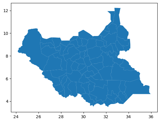
adm_boundaries.plot()
<Axes: >

get_summary?
Signature:
get_summary(
    gdf: geopandas.geodataframe.GeoDataFrame,
    spatial_join_method: Literal['touches', 'centroid', 'within'],
    fields: List[str],
    geometry: Optional[Literal['polygon', 'point']] = None,
) -> pandas.core.frame.DataFrame
Docstring:
Extract h3 level data from Space2Stats for a GeoDataFrame.

Parameters
----------
gdf : GeoDataFrame
    The Areas of Interest

spatial_join_method : ["touches", "centroid", "within"]
    The method to use for performing the spatial join between the AOI and H3 cells
        - "touches": Includes H3 cells that touch the AOI
        - "centroid": Includes H3 cells where the centroid falls within the AOI
        - "within": Includes H3 cells entirely within the AOI

fields : List[str]
    A list of field names to retrieve from the statistics table.

geometry : Optional["polygon", "point"]
    Specifies if the H3 geometries should be included in the response. It can be either "polygon" or "point". If None, geometries are not included

Returns
-------
DataFrame
    A DataFrame with the requested fields for each H3 cell that intersects with the AOIs.
File:      c:\users\wb514197\appdata\local\temp\ipykernel_33312\2584730817.py
Type:      function
Run API Calls
df = get_summary(
    gdf=adm_boundaries,
    spatial_join_method="centroid",
    fields=flood_vars,
    geometry="polygon"
)
pd.reset_option('display.max_colwidth')
df.head()
| shapeName | shapeISO | shapeID | shapeGroup | shapeType | index_gdf | index_h3 | hex_id | geometry | pop | pop_flood | pop_flood_pct | |
|---|---|---|---|---|---|---|---|---|---|---|---|---|
| 0 | Morobo | 79223893B16328156709571 | SSD | ADM2 | 0 | 0 | 866ae1067ffffff | {"type":"Polygon","coordinates":[[[30.62327290... | 4204.4385 | 609.631552 | 0.144997 | |
| 1 | Morobo | 79223893B16328156709571 | SSD | ADM2 | 0 | 1 | 866ae106fffffff | {"type":"Polygon","coordinates":[[[30.68007919... | 4776.9630 | 459.478346 | 0.096186 | |
| 2 | Morobo | 79223893B16328156709571 | SSD | ADM2 | 0 | 2 | 866ae114fffffff | {"type":"Polygon","coordinates":[[[30.61445415... | 3752.4004 | 341.734756 | 0.091071 | |
| 3 | Morobo | 79223893B16328156709571 | SSD | ADM2 | 0 | 3 | 866ae116fffffff | {"type":"Polygon","coordinates":[[[30.60563958... | 3304.6606 | 392.324178 | 0.118718 | |
| 4 | Morobo | 79223893B16328156709571 | SSD | ADM2 | 0 | 4 | 866ae132fffffff | {"type":"Polygon","coordinates":[[[30.84166572... | 7512.3320 | 865.229318 | 0.115175 |
Check that there are no duplicate hexagon ids
df['hex_id'].duplicated().sum()
0
Convert geometry column from geojson into shapely polygons
df["geometry"] = df["geometry"].apply(lambda geom: from_geojson(geom))
gdf = gpd.GeoDataFrame(df, geometry="geometry", crs="EPSG:4326")
gdf.head()
| shapeName | shapeISO | shapeID | shapeGroup | shapeType | index_gdf | index_h3 | hex_id | geometry | pop | pop_flood | pop_flood_pct | |
|---|---|---|---|---|---|---|---|---|---|---|---|---|
| 0 | Morobo | 79223893B16328156709571 | SSD | ADM2 | 0 | 0 | 866ae1067ffffff | POLYGON ((30.62327 3.62973, 30.63632 3.66096, ... | 4204.4385 | 609.631552 | 0.144997 | |
| 1 | Morobo | 79223893B16328156709571 | SSD | ADM2 | 0 | 1 | 866ae106fffffff | POLYGON ((30.68008 3.60768, 30.69312 3.63891, ... | 4776.9630 | 459.478346 | 0.096186 | |
| 2 | Morobo | 79223893B16328156709571 | SSD | ADM2 | 0 | 2 | 866ae114fffffff | POLYGON ((30.61445 3.68759, 30.6275 3.71879, 3... | 3752.4004 | 341.734756 | 0.091071 | |
| 3 | Morobo | 79223893B16328156709571 | SSD | ADM2 | 0 | 3 | 866ae116fffffff | POLYGON ((30.60564 3.7454, 30.61869 3.77659, 3... | 3304.6606 | 392.324178 | 0.118718 | |
| 4 | Morobo | 79223893B16328156709571 | SSD | ADM2 | 0 | 4 | 866ae132fffffff | POLYGON ((30.84167 3.59938, 30.85469 3.6306, 3... | 7512.3320 | 865.229318 | 0.115175 |
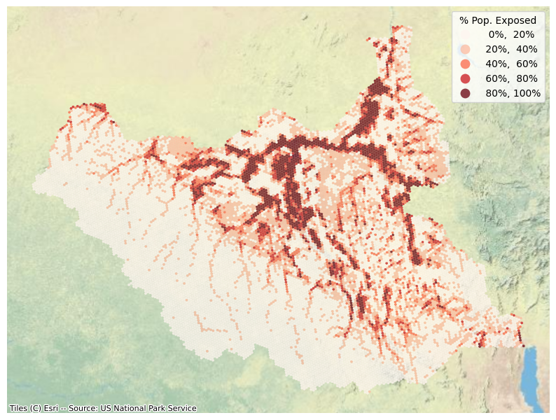
Map hexagon data
fig, ax = plt.subplots(1, 1, figsize=(10, 10))
gdf.plot(ax=ax, column="pop_flood_pct",
         legend=True, cmap="Reds", alpha=0.75,
         scheme="equal_interval", k=5,
         legend_kwds=dict(title='% Pop. Exposed', fmt="{:.0%}"),
         linewidth=0)
ctx.add_basemap(ax, source=ctx.providers.Esri.WorldPhysical, crs='EPSG:4326')
plt.axis("off")
plt.show()

Extract Admin Summaries#
adm_boundaries_zs = get_aggregate(
    gdf=adm_boundaries,
    spatial_join_method="centroid",
    fields=['pop', 'pop_flood'],
    aggregation_type="sum"
)
adm_boundaries_zs.head()
| shapeName | shapeISO | shapeID | shapeGroup | shapeType | geometry | pop | pop_flood | |
|---|---|---|---|---|---|---|---|---|
| 0 | Morobo | 79223893B16328156709571 | SSD | ADM2 | POLYGON ((30.56014 3.80448, 30.56025 3.80123, ... | 163323.45 | 18611.677807 | |
| 1 | Kajo-keji | 79223893B65724383376583 | SSD | ADM2 | POLYGON ((31.21043 4.02022, 31.09764 3.97353, ... | 323397.56 | 34155.373103 | |
| 2 | Lainya | 79223893B40788586970477 | SSD | ADM2 | POLYGON ((31.09684 3.73816, 31.097 3.738, 31.0... | 152762.36 | 17860.699796 | |
| 3 | Yei | 79223893B15931514297219 | SSD | ADM2 | POLYGON ((30.92897 3.92614, 30.92401 3.95754, ... | 338000.16 | 44152.720881 | |
| 4 | Juba | 79223893B61077901252755 | SSD | ADM2 | POLYGON ((31.72803 3.99162, 31.72429 4.00022, ... | 641935.60 | 99231.778778 |
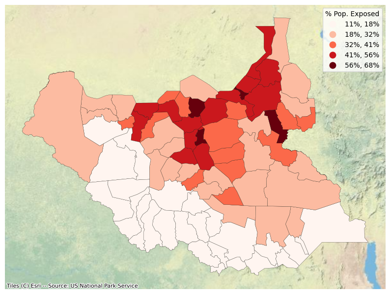
Recalculate share of population exposed with aggregate data
adm_boundaries_zs.loc[:, "pop_flood_pct"] = adm_boundaries_zs["pop_flood"] / adm_boundaries_zs["pop"]
fig, ax = plt.subplots(1, 1, figsize=(10, 10))
adm_boundaries_zs.plot(
    ax=ax, column="pop_flood_pct", legend=True,
    cmap="Reds", scheme="natural_breaks",
    k=5, legend_kwds=dict(title='% Pop. Exposed', fmt="{:.0%}"),
    linewidth=0.2, edgecolor='black')
ctx.add_basemap(ax, source=ctx.providers.Esri.WorldPhysical, crs='EPSG:4326')
plt.axis("off")
plt.show()

List top 20 provinces by population exposed
table = adm_boundaries_zs.sort_values('pop_flood_pct', ascending=False).head(20)[['shapeName', 'pop_flood', 'pop_flood_pct']].rename(
    columns={
        'shapeName': 'Province'
        })
table.loc[:, "Population Exposed"] = table.loc[:, "pop_flood"].apply(lambda x: f"{x:,.0f}")
table.loc[:, "Population Exposed (%)"] = table.loc[:, "pop_flood_pct"].apply(lambda x: f"{x:.2%}")
table.reset_index(drop=True, inplace=True)
display(table[['Province', 'Population Exposed', 'Population Exposed (%)']])
| Province | Population Exposed | Population Exposed (%) | |
|---|---|---|---|
| 0 | Guit | 39,438 | 68.05% |
| 1 | Ulang | 91,703 | 65.99% |
| 2 | Leer | 54,570 | 63.61% |
| 3 | Malakal | 103,890 | 61.19% |
| 4 | Mayom | 110,430 | 56.28% |
| 5 | Mayendit | 50,026 | 54.05% |
| 6 | Gogrial West | 152,568 | 53.71% |
| 7 | Panyijiar | 46,028 | 53.33% |
| 8 | Panyikang | 43,152 | 53.03% |
| 9 | Melut | 40,606 | 52.15% |
| 10 | Fangak | 87,145 | 51.88% |
| 11 | Fashoda | 34,966 | 51.53% |
| 12 | Manyo | 33,179 | 48.29% |
| 13 | Koch | 57,514 | 47.25% |
| 14 | Twic | 110,514 | 46.91% |
| 15 | Baliet | 40,963 | 45.50% |
| 16 | Rumbek North | 25,182 | 44.86% |
| 17 | Gogrial East | 51,352 | 41.18% |
| 18 | Luakpiny/Nasir | 133,452 | 41.08% |
| 19 | Aweil South | 30,248 | 40.88% |
