pop-x0.25

pop-x0.25#

Example

Dimensions#

This SEDAC population data has the dimensions:

time (datetime64[ns]) - The time dimension for the data, yearly resolution.
lat (float64) - The latitude dimension for the data, 1.0° resolution, based on raw data at 1/8° resolution.
lon (float64) - The longitude dimension for the data, 1.0° resolution, based on raw data at 1/8° resolution.
bnds (int64) - The bounds dimension for the data, [0, 1] for each coordinate.

Data variables are organized with respect to those dimensions and can be queried by index, or by dimension.

Example Data#

In the following section, we explore some sample data from the SEDAC dataset.

Reading the `.nc` file#

We use xarray, to read in the .nc file as an xarray.Dataset object.

import xarray as xr

data = xr.open_dataset("../timeseries-popdensity-annual-mean_pop-x1_gpw-v4-rev11-ssp370_timeseries_mean_2010-2100.nc")

Examining the data#

We can examine the data by printing the xarray.Dataset object. Specifically, we can see the dimensions, coordinates, and data variables.

Further examination of the data can be done by viewing an individual coordinate, data variable, or the attributes of the dataset.

data['time']

<xarray.DataArray 'time' (time: 10)>
array(['2010-07-01T00:00:00.000000000', '2020-07-01T00:00:00.000000000',
       '2030-07-01T00:00:00.000000000', '2040-07-01T00:00:00.000000000',
       '2050-07-01T00:00:00.000000000', '2060-07-01T00:00:00.000000000',
       '2070-07-01T00:00:00.000000000', '2080-07-01T00:00:00.000000000',
       '2090-07-01T00:00:00.000000000', '2100-07-01T00:00:00.000000000'],
      dtype='datetime64[ns]')
Coordinates:
  * time     (time) datetime64[ns] 2010-07-01 2020-07-01 ... 2100-07-01
Attributes:
    long_name:  time
    axis:       T

data['lon_bnds']

<xarray.DataArray 'lon_bnds' (lon: 361, bnds: 2)>
[722 values with dtype=float64]
Coordinates:
  * lon      (lon) float64 -180.0 -179.0 -178.0 -177.0 ... 178.0 179.0 180.0
Dimensions without coordinates: bnds

data.attrs

{'title': 'Gridded Population of the World, Version 4, Revision 11; 1x1-degrees based on 1/8th degree raw data',
 'data_source': 'Gridded Population of the World, Version 4: GPWv4; Revision 11, Dec 2018',
 'user': 'file standardized by Caspar Ammann, Climate Strategies',
 'creation_date': 'Thu Feb  9 09:26:42 MST 2023',
 'wb_truncation_label': 3,
 'wb_grid_label': 'x1',
 'wb_period_label': '2010-2100',
 'wb_percentile_label': 'mean',
 'wb_type_label': 'timeseries',
 'wb_model_label': 'gpw-v4',
 'wb_variant_label': 'rev11',
 'wb_scenario_label': 'ssp370',
 'wb_statistic_label': 'mean',
 'wb_aggregation_label': 'annual',
 'wb_variable_label': 'popdensity',
 'wb_product_label': 'timeseries',
 'wb_collection_label': 'pop-x1',
 'Source_Software': 'Esri ArcGIS',
 'Conventions': 'CF-1.0',
 'population_reference': " \nData Set: Jones, B., and B. C. O'Neill. 2020. Global One-Eighth Degree Population \nBase Year and Projection Grids Based on the Shared Socioeconomic Pathways, Revision 01.\nPalisades, NY: NASA Socioeconomic Data and Applications Center (SEDAC). \nhttps://doi.org/10.7927/m30p-j498. Accessed DAY MONTH YEAR\n \nScientific Publication: Jones, B., and B. C. O'Neill. 2016. Spatially Explicit Global \nPopulation Scenarios Consistent with the Shared Socioeconomic Pathways. \nEnvironmental Research Letters, 11 (2016): 084003. https://doi.org/10.1088/1748-9326/11/8/084003."}

Visualizing the data#

We can visualize the primary data variable in the example dataset, timeseries-popdensity-annual-mean (if matplotlib is installed), by using the built-in .plot() method of the xarray.DataArray object.

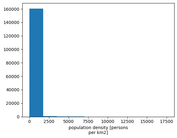
If we just call the .plot() method, we get a default plot of the data, which in this case reduces the dimensionality of the data from 3-D (time, lat, lon) to 1-D, by generating a bar plot of the mean value of the data variable over the entire time period for each latitude and longitude.

data['timeseries-popdensity-annual-mean'].plot()

(array([1.60643e+05, 5.12000e+02, 4.20000e+01, 2.90000e+01, 8.00000e+00,
        5.00000e+00, 6.00000e+00, 5.00000e+00, 7.00000e+00, 3.00000e+00]),
 array([    0.        ,  1760.3527832 ,  3520.70556641,  5281.05810547,
         7041.41113281,  8801.76367188, 10562.11621094, 12322.46875   ,
        14082.82226562, 15843.17480469, 17603.52734375]),
 <BarContainer object of 10 artists>)

../_images/e2b8482a47fd701ad36d817b754c84c1adaeee6451578a05b1490de459f2c1e0.png

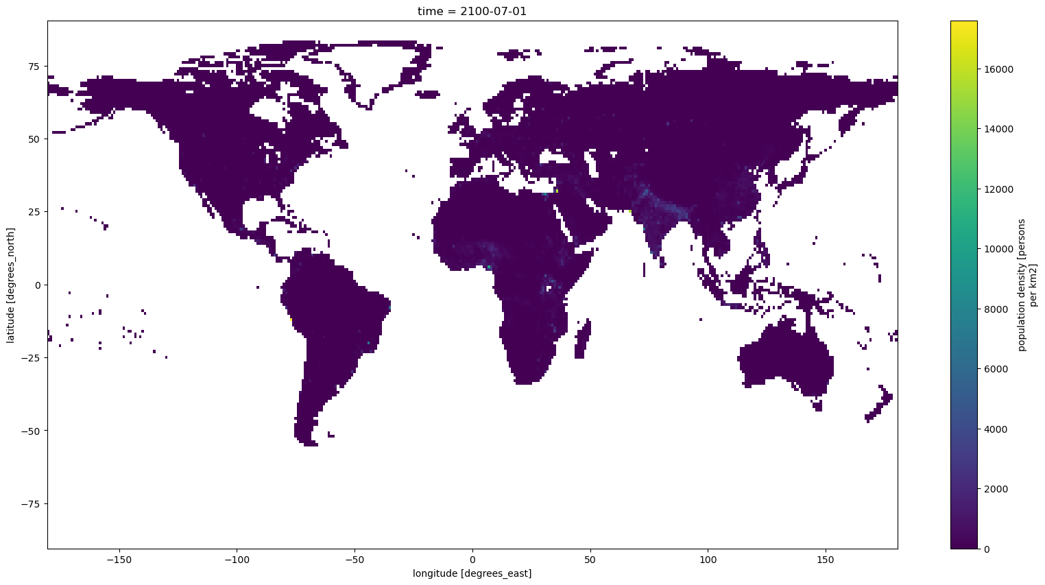
If we want to view the data as a 2-D surface plotted at a specific instance in time, we can use the .plot() method to specify the time index we want to plot. Because we are working with a .nc file that has been loaded as an xarray.Dataset object, we can use the .sel() method to select the time index we want to plot directly, we do not need to calculate or search for the index value.

data["timeseries-popdensity-annual-mean"].sel(time=slice('2100-07-01', '2100-07-01')).plot(figsize=(20,10))

<matplotlib.collections.QuadMesh at 0x7f075abbd760>

../_images/6da21a8e3e07d175d5884ffeda702690f9afa7bbf6b6a262e78a51db5f9b41b7.png