cru-x0.25 Example

Dimensions

The CRU data has the following dimensions:

• time (datetime64[ns]) - The time dimension for the data, monthly resolution.

• lat (float64) - The latitude dimension for the data, 0.5° resolution.

• lon (float64) - The longitude dimension for the data, 0.5° resolution.

• bnds (int64) - The bounds dimension for the data, [0, 1] for each coordinate.

Data variables are organized with respect to those dimensions and can be queried by index, or by dimension.

Example Data

In the following section, we explore some sample data from the CRU dataset.

Reading the .nc file

We use xarray, to read in the .nc file as an xarray.Dataset object.

import xarray as xr

data = xr.open_dataset("../climatology-tasmax-seasonal-mean_cru-x0.5_cru-ts4.07-historical_climatology_mean_1991-2020.nc")

Examining the data

We can examine the data by printing the xarray.Dataset object. Specifically, we can see the dimensions, coordinates, and data variables.

Further examination of the data can be done by viewing an individual coordinate, data variable, or the attributes of the dataset.

<xarray.Dataset>
Dimensions:                           (time: 4, lat: 360, lon: 720, bnds: 2)
Coordinates:
  * time                              (time) datetime64[ns] 1991-01-16 ... 19...
  * lat                               (lat) float32 -89.75 -89.25 ... 89.75
  * lon                               (lon) float32 -179.8 -179.2 ... 179.8
  * bnds                              (bnds) int32 0 1
Data variables:
    climatology-tasmax-seasonal-mean  (time, lat, lon) float32 ...
    lon_bnds                          (lon, bnds) float64 ...
    lat_bnds                          (lat, bnds) float64 ...
Attributes: (12/23)
    wb_truncation_label:   2
    wb_grid_label:         x0.5
    wb_period_label:       1991-2020
    wb_percentile_label:   mean
    wb_type_label:         climatology
    wb_model_label:        cru
    ...                    ...
    institution:           Data held at British Atmospheric Data Centre, RAL,...
    source:                Run ID = 2304141047. Data generated from:TMX deriv...
    history:               Fri 14 Apr 16:38:44 BST 2023 : User f098 : Program...
    references:            Information on the data is available at http://bad...
    comment:               Access to these data is available to any registere...
    contact:               support@ceda.ac.uk

xarray.Dataset

• Dimensions:
  • time: 4
  • lat: 360
  • lon: 720
  • bnds: 2
• Coordinates: (4)
  • time
    (time)
    datetime64[ns]
    1991-01-16 ... 1991-10-16

    typeConversion_op_ncl :

    double converted to float

    long_name :

    12 months of a climatological year

    axis :

    T

    standard_name :

    12 months of a climatological year

    climatology_period :

    1991-2020

    array(['1991-01-16T00:00:00.000000000', '1991-04-16T00:00:00.000000000',
           '1991-07-16T00:00:00.000000000', '1991-10-16T00:00:00.000000000'],
          dtype='datetime64[ns]')

  • lat
    (lat)
    float32
    -89.75 -89.25 ... 89.25 89.75

    bnds :

    lat_bnds

    units :

    degrees_north

    long_name :

    latitude

    bounds :

    lat_bnds

    axis :

    Y

    array([-89.75, -89.25, -88.75, ...,  88.75,  89.25,  89.75], dtype=float32)

  • lon
    (lon)
    float32
    -179.8 -179.2 ... 179.2 179.8

    bnds :

    lon_bnds

    units :

    degrees_east

    long_name :

    longitude

    bounds :

    lon_bnds

    axis :

    X

    array([-179.75, -179.25, -178.75, ...,  178.75,  179.25,  179.75],
          dtype=float32)

  • bnds
    (bnds)
    int32
    0 1

    long_name :

    grid bounds

    array([0, 1], dtype=int32)

• Data variables: (3)
  • climatology-tasmax-seasonal-mean
    (time, lat, lon)
    float32
    ...

    climatoloyg_calculation :

    avg

    valid_max :

    45.735943

    valid_min :

    -43.066257

    seaonal_calculation :

    avg

    correlation_decay_distance :

    1200.0

    units :

    degC

    long_name :

    near-surface temperature maximum

    [1036800 values with dtype=float32]

  • lon_bnds
    (lon, bnds)
    float64
    ...

    long_name :

    longitude bounds

    [1440 values with dtype=float64]

  • lat_bnds
    (lat, bnds)
    float64
    ...

    long_name :

    latitude bounds

    [720 values with dtype=float64]

• Indexes: (4)
  • time
    PandasIndex

    PandasIndex(DatetimeIndex(['1991-01-16', '1991-04-16', '1991-07-16', '1991-10-16'], dtype='datetime64[ns]', name='time', freq=None))

  • lat
    PandasIndex

    PandasIndex(Index([-89.75, -89.25, -88.75, -88.25, -87.75, -87.25, -86.75, -86.25, -85.75,
           -85.25,
           ...
            85.25,  85.75,  86.25,  86.75,  87.25,  87.75,  88.25,  88.75,  89.25,
            89.75],
          dtype='float32', name='lat', length=360))

  • lon
    PandasIndex

    PandasIndex(Index([-179.75, -179.25, -178.75, -178.25, -177.75, -177.25, -176.75, -176.25,
           -175.75, -175.25,
           ...
            175.25,  175.75,  176.25,  176.75,  177.25,  177.75,  178.25,  178.75,
            179.25,  179.75],
          dtype='float32', name='lon', length=720))

  • bnds
    PandasIndex

    PandasIndex(Index([0, 1], dtype='int32', name='bnds'))

• Attributes: (23)

  wb_truncation_label :

  2

  wb_grid_label :

  x0.5

  wb_period_label :

  1991-2020

  wb_percentile_label :

  mean

  wb_type_label :

  climatology

  wb_model_label :

  cru

  wb_variant_label :

  ts4.07

  wb_scenario_label :

  historical

  wb_statistic_label :

  mean

  wb_aggregation_label :

  seasonal

  wb_variable_label :

  tasmax

  wb_product_label :

  climatology

  wb_collection_label :

  cru-x0.5

  wb :

  wb_access_citation = Please acknowledge data source as : Climatic Research Unit (University of East Anglia) and Met Office accessed through: World Bank Climate Change Knowledge Portal : https://climateknowledgeportal.worldbank.org wb_data_license_comment = data available under UK Open Government License: https://www.nationalarchives.gov.uk/doc/open-government-licence/version/3/ wb_data_comment = Processed CRU data by WB; RAW-data contact: support@ceda.ac.uk wb_scientific_reference = Harris, I., Osborn, T.J., Jones, P. et al. Version 4 of the CRU TS monthly high-resolution gridded multivariate climate dataset. Sci Data 7, 109 (2020). https://doi.org/10.1038/s41597-020-0453-3 wb_author = Dr. Caspar M Ammann, Climate Strategies, ammann@climatestrategies.com

  wb_OBS :

  wb_creation_date = Fri Sep 1 02:32:28 PM MDT 2023 wb_OBS_version = 2.0 (summer 2022)

  Conventions :

  CF-1.4

  title :

  CRU TS4.07 Maximum Temperature

  institution :

  Data held at British Atmospheric Data Centre, RAL, UK.

  source :

  Run ID = 2304141047. Data generated from:TMX derived from gridded TMP & DTR absolutes, DTR in turn derived from tmn.2304141039.dtb, tmx.2304141039.dtb

  history :

  Fri 14 Apr 16:38:44 BST 2023 : User f098 : Program makegridsauto.for called by update.for

  references :

  Information on the data is available at http://badc.nerc.ac.uk/data/cru/

  comment :

  Access to these data is available to any registered CEDA user.

  contact :

  support@ceda.ac.uk

data['time']

<xarray.DataArray 'time' (time: 4)>
array(['1991-01-16T00:00:00.000000000', '1991-04-16T00:00:00.000000000',
       '1991-07-16T00:00:00.000000000', '1991-10-16T00:00:00.000000000'],
      dtype='datetime64[ns]')
Coordinates:
  * time     (time) datetime64[ns] 1991-01-16 1991-04-16 1991-07-16 1991-10-16
Attributes:
    typeConversion_op_ncl:  double converted to float
    long_name:              12 months of a climatological year
    axis:                   T
    standard_name:          12 months of a climatological year
    climatology_period:     1991-2020

xarray.DataArray

'time'

• time: 4

• 1991-01-16 1991-04-16 1991-07-16 1991-10-16

  array(['1991-01-16T00:00:00.000000000', '1991-04-16T00:00:00.000000000',
         '1991-07-16T00:00:00.000000000', '1991-10-16T00:00:00.000000000'],
        dtype='datetime64[ns]')

• Coordinates: (1)
  • time
    (time)
    datetime64[ns]
    1991-01-16 ... 1991-10-16

    typeConversion_op_ncl :

    double converted to float

    long_name :

    12 months of a climatological year

    axis :

    T

    standard_name :

    12 months of a climatological year

    climatology_period :

    1991-2020

    array(['1991-01-16T00:00:00.000000000', '1991-04-16T00:00:00.000000000',
           '1991-07-16T00:00:00.000000000', '1991-10-16T00:00:00.000000000'],
          dtype='datetime64[ns]')

• Indexes: (1)
  • time
    PandasIndex

    PandasIndex(DatetimeIndex(['1991-01-16', '1991-04-16', '1991-07-16', '1991-10-16'], dtype='datetime64[ns]', name='time', freq=None))

• Attributes: (5)

  typeConversion_op_ncl :

  double converted to float

  long_name :

  12 months of a climatological year

  axis :

  T

  standard_name :

  12 months of a climatological year

  climatology_period :

  1991-2020

data['lon_bnds']

<xarray.DataArray 'lon_bnds' (lon: 720, bnds: 2)>
[1440 values with dtype=float64]
Coordinates:
  * lon      (lon) float32 -179.8 -179.2 -178.8 -178.2 ... 178.8 179.2 179.8
  * bnds     (bnds) int32 0 1
Attributes:
    long_name:  longitude bounds

xarray.DataArray

'lon_bnds'

• lon: 720
• bnds: 2

• ...

  [1440 values with dtype=float64]

• Coordinates: (2)
  • lon
    (lon)
    float32
    -179.8 -179.2 ... 179.2 179.8

    bnds :

    lon_bnds

    units :

    degrees_east

    long_name :

    longitude

    bounds :

    lon_bnds

    axis :

    X

    array([-179.75, -179.25, -178.75, ...,  178.75,  179.25,  179.75],
          dtype=float32)

  • bnds
    (bnds)
    int32
    0 1

    long_name :

    grid bounds

    array([0, 1], dtype=int32)

• Indexes: (2)
  • lon
    PandasIndex

    PandasIndex(Index([-179.75, -179.25, -178.75, -178.25, -177.75, -177.25, -176.75, -176.25,
           -175.75, -175.25,
           ...
            175.25,  175.75,  176.25,  176.75,  177.25,  177.75,  178.25,  178.75,
            179.25,  179.75],
          dtype='float32', name='lon', length=720))

  • bnds
    PandasIndex

    PandasIndex(Index([0, 1], dtype='int32', name='bnds'))

• Attributes: (1)

  long_name :

  longitude bounds

data.attrs

{'wb_truncation_label': 2,
 'wb_grid_label': 'x0.5',
 'wb_period_label': '1991-2020',
 'wb_percentile_label': 'mean',
 'wb_type_label': 'climatology',
 'wb_model_label': 'cru',
 'wb_variant_label': 'ts4.07',
 'wb_scenario_label': 'historical',
 'wb_statistic_label': 'mean',
 'wb_aggregation_label': 'seasonal',
 'wb_variable_label': 'tasmax',
 'wb_product_label': 'climatology',
 'wb_collection_label': 'cru-x0.5',
 'wb': ' \nwb_access_citation = Please acknowledge data source as :\n   Climatic Research Unit (University of East Anglia) and Met Office\n   accessed through: World Bank Climate Change Knowledge Portal : https://climateknowledgeportal.worldbank.org \nwb_data_license_comment = data available under UK Open Government License: https://www.nationalarchives.gov.uk/doc/open-government-licence/version/3/\nwb_data_comment = Processed CRU data by WB; RAW-data contact: support@ceda.ac.uk\nwb_scientific_reference = Harris, I., Osborn, T.J., Jones, P. et al.\n   Version 4 of the CRU TS monthly high-resolution gridded multivariate climate dataset.\n   Sci Data 7, 109 (2020). https://doi.org/10.1038/s41597-020-0453-3\nwb_author = Dr. Caspar M Ammann, Climate Strategies, ammann@climatestrategies.com',
 'wb_OBS': ' \nwb_creation_date = Fri Sep  1 02:32:28 PM MDT 2023\nwb_OBS_version = 2.0 (summer 2022)',
 'Conventions': 'CF-1.4',
 'title': 'CRU TS4.07 Maximum Temperature',
 'institution': 'Data held at British Atmospheric Data Centre, RAL, UK.',
 'source': 'Run ID = 2304141047. Data generated from:TMX derived from gridded TMP & DTR absolutes, DTR in turn derived from tmn.2304141039.dtb, tmx.2304141039.dtb',
 'history': 'Fri 14 Apr 16:38:44 BST 2023 : User f098 : Program makegridsauto.for called by update.for',
 'references': 'Information on the data is available at http://badc.nerc.ac.uk/data/cru/',
 'comment': 'Access to these data is available to any registered CEDA user.',
 'contact': 'support@ceda.ac.uk'}

Visualizing the data

We can visualize the primary data variable in the example dataset, climatology-tasmax-seasonal-mean (if matplotlib is installed), by using the built-in .plot() method of the xarray.DataArray object.

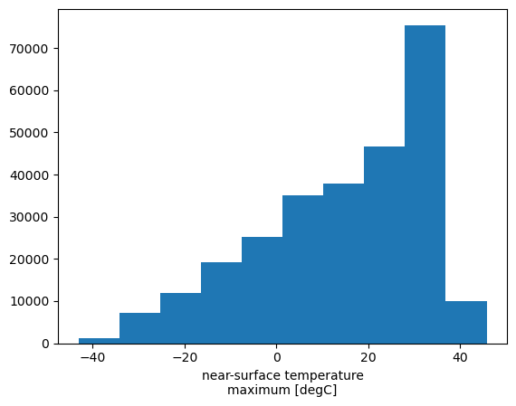
If we just call the .plot() method, we get a default plot of the data, which in this case reduces the dimensionality of the data from 3-D (time, lat, lon) to 1-D, by generating a bar plot of the mean value of the data variable over the entire time period for each latitude and longitude.

# visualize the data
data['climatology-tasmax-seasonal-mean'].plot()

(array([ 1161.,  7122., 11847., 19200., 25246., 35081., 37935., 46660.,
        75466.,  9962.]),
 array([-43.06625748, -34.18603897, -25.30581665, -16.42559814,
         -7.54537725,   1.33484268,  10.2150631 ,  19.09528351,
         27.97550201,  36.85572433,  45.73594284]),
 <BarContainer object of 10 artists>)

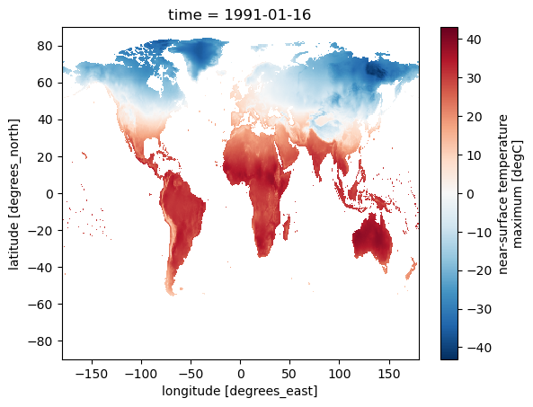
If we want to view the data as a 2-D surface plotted at a specific instance in time, we can use the .plot() method to specify the time index we want to plot. Because we are working with a .nc file that has been loaded as an xarray.Dataset object, we can use the .sel() method to select the time index we want to plot directly, we do not need to calculate or search for the index value.

# surface plot of the data
data['climatology-tasmax-seasonal-mean'].sel(time='1991-01-16').plot()

<matplotlib.collections.QuadMesh at 0x7f98fd71b320>