cmip6-x0.25 Example

cmip6-x0.25 Example#

Dimensions#

The CMIP6 data has the following dimensions:

time (datetime64[ns]) - The time dimension for the data, monthly resolution.
lat (float64) - The latitude dimension for the data, 0.25° resolution.
lon (float64) - The longitude dimension for the data, 0.25° resolution.
bnds (int64) - The bounds dimension for the data, [0, 1] for each coordinate.

Data variables are organized with respect to those dimensions and can be queried by index, or by dimension.

Example Data#

In the following section, we explore some sample data from the CRU dataset.

Reading the `.nc` file#

We use xarray, to read in the .nc file as an xarray.Dataset object.

import xarray as xr

data = xr.open_dataset("../climatology-tr-monthly-mean_cmip6-x0.25_hadgem3-gc31-mm-r1i1p1f3-ssp126_climatology_mean_2040-2059.nc")

Examining the data#

We can examine the data by printing the xarray.Dataset object. Specifically, we can see the dimensions, coordinates, and data variables.

Further examination of the data can be done by viewing an individual coordinate, data variable, or the attributes of the dataset.

data['time']

<xarray.DataArray 'time' (time: 12)>
array(['2040-01-16T00:00:00.000000000', '2040-02-16T00:00:00.000000000',
       '2040-03-16T00:00:00.000000000', '2040-04-16T00:00:00.000000000',
       '2040-05-16T00:00:00.000000000', '2040-06-16T00:00:00.000000000',
       '2040-07-16T00:00:00.000000000', '2040-08-16T00:00:00.000000000',
       '2040-09-16T00:00:00.000000000', '2040-10-16T00:00:00.000000000',
       '2040-11-16T00:00:00.000000000', '2040-12-16T00:00:00.000000000'],
      dtype='datetime64[ns]')
Coordinates:
  * time     (time) datetime64[ns] 2040-01-16 2040-02-16 ... 2040-12-16
Attributes:
    long_name:           12 months of a climatological year
    axis:                T
    standard_name:       12 months of a climatological year
    climatology_period:  2040-2059

data.attrs

{'wb_truncation_label': 1,
 'wb_grid_label': 'x0.25',
 'wb_period_label': '2040-2059',
 'wb_percentile_label': 'mean',
 'wb_type_label': 'climatology',
 'wb_model_label': 'hadgem3-gc31-mm',
 'wb_variant_label': 'r1i1p1f3',
 'wb_scenario_label': 'ssp126',
 'wb_statistic_label': 'mean',
 'wb_aggregation_label': 'monthly',
 'wb_variable_label': 'tr',
 'wb_product_label': 'climatology',
 'wb_collection_label': 'cmip6-x0.25',
 'wb': " \nwb_data_citation = Please acknowledge data source as :\n   World Bank Climate Change Knowledge Portal : https://climateknowledgeportal.worldbank.org \nwb_ensemble_citation = Please acknowledge CMIP6 multi-model ensemble data source as : \n   World Bank Climate Change Knowledge Portal : https://climateknowledgeportal.worldbank.org. \nwb_cmip6_acknowledgement = We acknowledge the World Climate Research Programme, which, through its Working Group \n   on Coupled Modeling, coordinated and promoted CMIP6. We thank the climate modeling groups \n   for producing and making available their model output, the Earth System Grid Federation (ESGF)\n   for archiving the data and providing access, and the multiple funding agencies who support CMIP6 and ESGF.\nwb_cmip6_terms_of_use = All CMIP6 GCM model inputs, as noted in Table 1, and any derivatives work, such as this dataset,\n   are governed by the original Terms of use (https://pcmdi.llnl.gov/CMIP6/TermsOfUse/TermsOfUse6-1.html)\n   and may have some restrictions on usage. See the individual netcdf files for the data licensing,\n   the global attribute cmip6_license notes the specific license the data may fall under.\nwb_general_warning = The CMIP6 archive contains the output of scientific simulations of the past and projected \n   futures that are subject to multiple sources of error, ranging from errors in the data handling, \n   to errors in the representation of the real world in either the model, or the experimental setup \n   for which the model was used. Different parts of the CMIP6 archive may be subject to differing \n   levels of such errors, and users should be alert to these issues, and their potential consequences \n   (and to the limitations of liability expressed in the data license). \nwb_grid = regridded to common resolution (x1: 180x360; x0.5: 360x720; x0.25 721x1440) \nwb_CMIP6_reference = Eyring, V., S. Bony, G.A. Meehl, C.A. Senior, B. Stevens, R.J. Stouffer, and K.E. Taylor, 2016: \n   Overview of the Coupled Model Intercomparison Project Phase 6 (CMIP6) experimental design and organization. \n   Geosci. Model Dev., 9, 1937-1958, 2016. https://doi.org/10.5194/gmd-9-1937-2016. \nwb_ScenarioMIP_reference = O'Neill, B.C., Tebaldi, C., van Vuuren, D.P., Eyring, V., Friedlingstein, P., Hurtt, G., Knutti, R., \n   Kriegler, E., Lamarque, J.-F., Lowe, J., Meehl, G.A., Moss, R., Riahi, K., and Sanderson, B.M.: \n   The Scenario Model Intercomparison Project (ScenarioMIP) for CMIP6,  \n   Geosci. Model Dev., 9, 3461-3482, 1016. doi:10.5194/gmd-9-3461-2016. \nwb_author = Dr. Caspar M Ammann, Climate Strategies, ammann@climatestrategies.com\nwb_downscaling_source = NASA Earth Exchange (NEX) Global Daily Downscaled Projections (GDDP): \n   [https://doi.org/10.7917/OFSG3345; Described in : \n   Thrasher, B., Wang, W., Michaelis, A. et al. NASA Global Daily Downscaled Projections, CMIP6. \n      Sci Data 9, 262 (2022). https://doi.org/10.1038/s41597-022-01393-4\n   Thrasher, B., Wang, W., Michaelis, A. Nemani, R. (2021). NEX-GDDP-CMIP6.\n      NASA Center for Climate Simulation. https://doi.org/10.7917/OFSG3345\n   based on methods described in: \n   Thrasher, B., Maurer, E. P., McKellar, C., & Duffy, P. B., 2012: Technical Note:\n      Bias correcting climate model simulated daily temperature extremes with quantile mapping.\n      Hydrology and Earth System Sciences, 16(9), 3309-3314, doi:10.5194/hess-16-3309-2012.\nwb_downscaling_author = Dr. Bridget Thrasher, bridget@climateanalyticsgroup.org\nwb_CMIP6_license = Creative Commons Zero license (CC0) license, \n   see https://wcrp-cmip.github.io/CMIP6_CVs/docs/CMIP6_source_id_licenses.html)\nwb_downscaling_acknowledgement = Climate scenarios used were from the NEX-GDDP-CMIP6 dataset, \n   prepared by the Climate Analytics Group and NASA Ames Research Center using\n   the NASA Earth Exchange and distributed by the NASA Center for Climate Simulation (NCCS).",
 'wb_CMIP6': ' \nwb_creation_date = Fri Mar 17 13:41:19 PDT 2023\nwb_CMIP6_version = 3.0 (winter 2022/2023)'}

Visualizing the data#

We can visualize the primary data variable in the example dataset, climatology-tr-monthly-mean (if matplotlib is installed), by using the built-in .plot() method of the xarray.DataArray object.

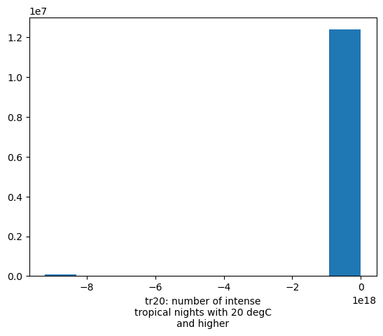
If we just call the .plot() method, we get a default plot of the data, which in this case reduces the dimensionality of the data from 3-D (time, lat, lon) to 1-D, by generating a bar plot of the mean value of the data variable over the entire time period for each latitude and longitude.

# visualize the data
data['climatology-tr-monthly-mean'].astype(float).plot()

(array([   69120.,        0.,        0.,        0.,        0.,        0.,
               0.,        0.,        0., 12389760.]),
 array([-9.22337204e+18, -8.30077563e+18, -7.37817923e+18, -6.45558283e+18,
        -5.53298642e+18, -4.61039002e+18, -3.68779361e+18, -2.76519721e+18,
        -1.84260081e+18, -9.20004404e+17,  2.59200000e+15]),
 <BarContainer object of 10 artists>)

../_images/ef54c68fd5ea46ecf1ec15cac5fdb916d0619343d7e4acfce018c872e09e51a1.png

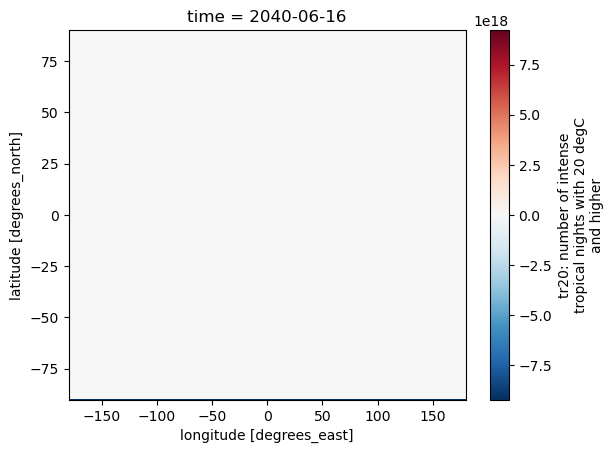
If we want to view the data as a 2-D surface plotted at a specific instance in time, we can use the .plot() method to specify the time index we want to plot. Because we are working with a .nc file that has been loaded as an xarray.Dataset object, we can use the .sel() method to select the time index we want to plot directly, we do not need to calculate or search for the index value.

# surface plot of the data
data['climatology-tr-monthly-mean'].sel(time='2040-06-16').astype(float).plot()

<matplotlib.collections.QuadMesh at 0x7fa36f775b50>

../_images/84670769a876a5e71472930912901a03a1196a23f761f9baeed083b4f2a23e87.png