Assessing Quality of Nighttime Lights Data • blackmarbler

Overview

The quality of nighttime lights data can be impacted by a number of factors, particularly cloud cover. To facilitate analysis using high quality data, Black Marble (1) marks the quality of each pixel and (2) in some cases, uses data from a previous date to fill the value—using a temporally-gap filled NTL value.

This page illustrates how to examine the quality of nighttime lights data.

Setup
Daily data
Monthly/annual data

Setup

We first load packages and obtain a polygon for a region of interest; for this example, we use Switzerland.

library(blackmarbler)
library(geodata)
library(sf)
library(raster)
library(ggplot2)
library(tidyterra)
library(dplyr)
library(exactextractr)
library(lubridate)
library(tidyr)
library(geodata)
library(knitr)

bearer <- "BEARER-TOKEN-HERE"

roi_sf <- gadm(country = "CHE", level=0, path = tempdir()) |> st_as_sf()

Daily Data

Below shows an example examining quality for daily data (VNP46A2).

Gap filled nighttime lights

We download data for January 1st, 2023. When the variable parameter is not specified, bm_raster creates a raster using the Gap_Filled_DNB_BRDF-Corrected_NTL variable for daily data. This variable “gap fills” poor quality observations (ie, pixels with cloud cover) using data from previous days.

ntl_r <- bm_raster(roi_sf = roi_sf,
                   product_id = "VNP46A2",
                   date = "2023-01-01",
                   bearer = bearer,
                   variable = "Gap_Filled_DNB_BRDF-Corrected_NTL")

Show code to produce map

#### Prep data
ntl_m_r <- ntl_r |> terra::mask(roi_sf) 

## Distribution is skewed, so log
ntl_m_r[] <- log(ntl_m_r[]+1)

##### Map 
ggplot() +
  geom_spatraster(data = ntl_m_r) +
  scale_fill_gradient2(low = "black",
                       mid = "yellow",
                       high = "red",
                       midpoint = 4,
                       na.value = "transparent") +
  coord_sf() + 
  theme_void() +
  theme(plot.title = element_text(face = "bold", hjust = 0.5),
        legend.position = "none")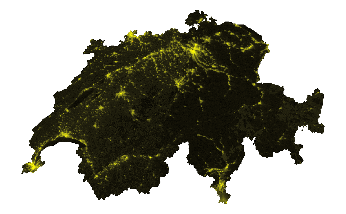

The Latest_High_Quality_Retrieval indicates the number of days since the current date that the nighttime lights value comes from for gap filling.

ntl_tmp_gap_r <- bm_raster(roi_sf = roi_sf,
                           product_id = "VNP46A2",
                           date = "2023-01-01",
                           bearer = bearer,
                           variable = "Latest_High_Quality_Retrieval")

Show code to produce map

#### Prep data
ntl_tmp_gap_r <- ntl_tmp_gap_r |> terra::mask(roi_sf) 

##### Map 
ggplot() +
  geom_spatraster(data = ntl_tmp_gap_r) +
  scale_fill_distiller(palette = "Spectral",
                       na.value = "transparent") +
  coord_sf() + 
  theme_void() +
  labs(fill = "Temporal\nGap\n(Days)",
       title = "Temporal gap between date (Jan 1, 2023)\nand date of high quality pixel used") +
  theme(plot.title = element_text(face = "bold", hjust = 0.5))

Non gap filled nighttime lights

Instead of using gap-filled data, we could also just use nighttime light values from the date selected using the DNB_BRDF-Corrected_NTL variable.

ntl_r <- bm_raster(roi_sf = roi_sf,
                   product_id = "VNP46A2",
                   date = "2023-01-01",
                   bearer = bearer,
                   variable = "DNB_BRDF-Corrected_NTL")

Show code to produce map

#### Prep data
ntl_m_r <- ntl_r |> terra::mask(roi_sf) 

## Distribution is skewed, so log
ntl_m_r[] <- log(ntl_m_r[] + 1)

##### Map 
ggplot() +
  geom_spatraster(data = ntl_m_r) +
  scale_fill_gradient2(low = "black",
                       mid = "yellow",
                       high = "red",
                       midpoint = 4,
                       na.value = "transparent") +
  coord_sf() + 
  theme_void() +
  theme(plot.title = element_text(face = "bold", hjust = 0.5),
        legend.position = "none")

We notice that a number of observations are missing. To understand the extent of missing date, we can use the following code to determine (1) the total number of pixels that cover Switzerland, (2) the total number of non-NA nighttime light pixels, and (3) the proportion of non-NA pixels.

n_pixel <- function(values, coverage_fraction){
  length(values)
}

n_non_na_pixel <- function(values, coverage_fraction){
  sum(!is.na(values))
}

n_pixel_num        <- exact_extract(ntl_r, roi_sf, n_pixel)
n_non_na_pixel_num <- exact_extract(ntl_r, roi_sf, n_non_na_pixel)

print(n_pixel_num)
#> [1] 282934
print(n_non_na_pixel_num)
#> [1] 122035
print(n_non_na_pixel_num / n_pixel_num)
#> [1] 0.4313197

By default, the bm_extract function computes these values:

ntl_df <- bm_extract(roi_sf = roi_sf,
                     product_id = "VNP46A2",
                   date = seq.Date(from = ymd("2023-01-01"),
                                   to = ymd("2023-01-10"),
                                   by = 1),
                   bearer = bearer,
                   variable = "DNB_BRDF-Corrected_NTL")

knitr::kable(ntl_df)

The below figure shows trends in average nighttime lights (left) and the proportion of the country with a value for nighttime lights (right). For some days, low number of pixels corresponds to low nighttime lights (eg, January 3 and 5th); however, for other days, low number of pixels corresponds to higher nighttime lights (eg, January 9 and 10). On January 3 and 5, missing pixels could have been over typically high-lit areas (eg, cities)—while on January 9 and 10, missing pixels could have been over typically lower-lit areas.

Show code to produce figure


ntl_df %>%
  dplyr::select(date, ntl_mean, prop_non_na_pixels) %>%
  pivot_longer(cols = -date) %>%
  
  ggplot(aes(x = date,
             y = value)) + 
  geom_line() +
  facet_wrap(~name,
             scales = "free")

Quality

For daily data, the quality values are:

0: High-quality, Persistent nighttime lights
1: High-quality, Ephemeral nighttime Lights
2: Poor-quality, Outlier, potential cloud contamination, or other issues

We can map quality by using the Mandatory_Quality_Flag variable.

quality_r <- bm_raster(roi_sf = roi_sf,
                       product_id = "VNP46A2",
                       date = "2023-01-01",
                       bearer = bearer,
                       variable = "Mandatory_Quality_Flag")

Show code to produce map

#### Prep data
quality_r <- quality_r |> terra::mask(roi_sf) 

qual_levels <- data.frame(id=0:2, cover=c("0: High-quality, persistent", 
                                  "1: High-quality, ephemeral", 
                                  "2: Poor-quality"))

levels(quality_r) <- qual_levels

##### Map 
ggplot() +
  geom_spatraster(data = quality_r) +
  scale_fill_brewer(palette = "Spectral", 
                    direction = -1,
                    na.value = "transparent") + 
  labs(fill = "Quality") +
  coord_sf() + 
  theme_void() +
  theme(plot.title = element_text(face = "bold", hjust = 0.5))

Nighttime lights for good quality observations

The quality_flag_rm parameter determines which pixels are set to NA based on the quality indicator. By default, no pixels are filtered out (except for those that are assigned a “fill value” by BlackMarble, which are always removed). However, if we only want data for good quality pixels, we can adjust the quality_flag_rm parameter.

ntl_good_qual_r <- bm_raster(roi_sf = roi_sf,
                             product_id = "VNP46A2", 
                             date = "2023-01-01",
                             bearer = bearer,
                             variable = "DNB_BRDF-Corrected_NTL",
                             quality_flag_rm = 2)

Show code to produce map

#### Prep data
ntl_good_qual_r <- ntl_good_qual_r |> terra::mask(roi_sf) 

## Distribution is skewed, so log
ntl_good_qual_r[] <- log(ntl_good_qual_r[]+1)

##### Map 
ggplot() +
  geom_spatraster(data = ntl_good_qual_r) +
  scale_fill_gradient2(low = "black",
                       mid = "yellow",
                       high = "red",
                       midpoint = 4,
                       na.value = "transparent") +
  coord_sf() + 
  theme_void() +
  theme(plot.title = element_text(face = "bold", hjust = 0.5),
        legend.position = "none")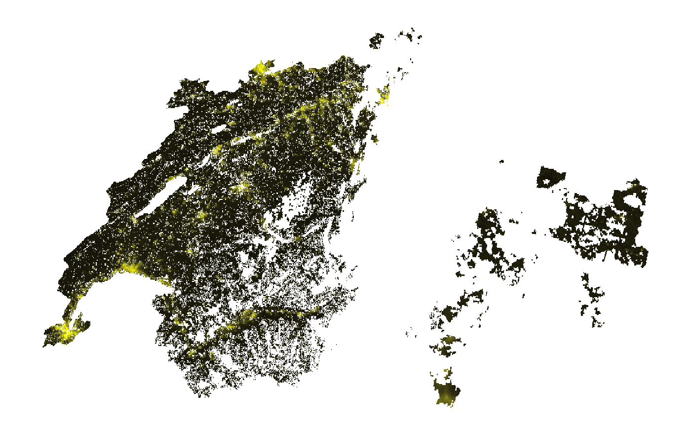

Monthly/Annual Data

Below shows an example examining quality for monthly data (VNP46A3). The same approach can be used for annual data (VNP46A4); the variables are the same for both monthly and annual data.

Nighttime Lights

We download data for January 2023. When the variable parameter is not specified, bm_raster creates a raster using the NearNadir_Composite_Snow_Free variable for monthly and annual data—which is nighttime lights, removing effects from snow cover.

ntl_r <- bm_raster(roi_sf = roi_sf,
                   product_id = "VNP46A3", 
                   date = "2023-01-01",
                   bearer = bearer,
                   variable = "NearNadir_Composite_Snow_Free")

Show code to produce map

#### Prep data
ntl_r <- ntl_r |> terra::mask(roi_sf) 

## Distribution is skewed, so log
ntl_r[] <- log(ntl_r[] + 1)

##### Map 
ggplot() +
  geom_spatraster(data = ntl_r) +
  scale_fill_gradient2(low = "black",
                       mid = "yellow",
                       high = "red",
                       midpoint = 4,
                       na.value = "transparent") +
  coord_sf() + 
  theme_void() +
  theme(plot.title = element_text(face = "bold", hjust = 0.5),
        legend.position = "none")

Number of Observations

Black Marble removes poor quality observations, such as pixels covered by clouds. To determine the number of observations used to generate nighttime light values for each pixel, we add _Num to the variable name.

cf_r <- bm_raster(roi_sf = roi_sf,
                  product_id = "VNP46A3",
                  date = "2023-01-01",
                  bearer = bearer,
                  variable = "NearNadir_Composite_Snow_Free_Num")

Show code to produce map

#### Prep data
cf_r <- cf_r |> terra::mask(roi_sf) 

##### Map 
ggplot() +
  geom_spatraster(data = cf_r) +
  scale_fill_viridis_c(na.value = "transparent") + 
  labs(fill = "Number of\nObservations") +
  coord_sf() + 
  theme_void() +
  theme(plot.title = element_text(face = "bold", hjust = 0.5))

Quality

For monthly and annual data, the quality values are:

0: Good-quality, The number of observations used for the composite is larger than 3
1: Poor-quality, The number of observations used for the composite is less than or equal to 3
2: Gap filled NTL based on historical data

We can map quality by adding _Quality to the variable name.

quality_r <- bm_raster(roi_sf = roi_sf,
                       product_id = "VNP46A3",
                       date = "2023-01-01",
                       bearer = bearer,
                       variable = "NearNadir_Composite_Snow_Free_Quality")

Show code to produce map

#### Prep data
quality_r <- quality_r |> terra::mask(roi_sf) 

qual_levels <- data.frame(id=0:2, cover=c("0: Good quality", 
                                  "1: Poor quality", 
                                  "2: Gap filled"))

levels(quality_r) <- qual_levels

##### Map 
ggplot() +
  geom_spatraster(data = quality_r) +
  scale_fill_brewer(palette = "Spectral", 
                    direction = -1,
                    na.value = "transparent") + 
  labs(fill = "Quality") +
  coord_sf() + 
  theme_void() +
  theme(plot.title = element_text(face = "bold", hjust = 0.5))

Nighttime lights for good quality observations

The quality_flag_rm parameter determines which pixels are set to NA based on the quality indicator. By default, no pixels are filtered out (except for those that are assigned a “fill value” by BlackMarble, which are always removed). However, if we also want to remove poor quality pixels and remove pixels that are gap filled, we can adjust the quality_flag_rm parameter.

ntl_good_qual_r <- bm_raster(roi_sf = roi_sf,
                             product_id = "VNP46A3", 
                             date = "2023-01-01",
                             bearer = bearer,
                             variable = "NearNadir_Composite_Snow_Free",
                             quality_flag_rm = c(1,2)) # 1 = poor quality; 2 = gap filled based on historical data

Show code to produce map

#### Prep data
ntl_good_qual_r <- ntl_good_qual_r |> terra::mask(roi_sf) 

## Distribution is skewed, so log
ntl_good_qual_r[] <- log(ntl_good_qual_r[] + 1)

##### Map 
ggplot() +
  geom_spatraster(data = ntl_good_qual_r) +
  scale_fill_gradient2(low = "black",
                       mid = "yellow",
                       high = "red",
                       midpoint = 4,
                       na.value = "transparent") +
  coord_sf() + 
  theme_void() +
  theme(plot.title = element_text(face = "bold", hjust = 0.5),
        legend.position = "none")