Chapter 2 Technical Documentation of SPI Indicators
2.1 Data Use
Cleaning for Data Use Indicators. Data Use (5 Indicators):
- 1.1_DUNL - Indicator 1.1: Data use by national legislature
- 1.2_DUNE - Indicator 1.2: Data use by national executive branch
- 1.3_DUCS - Indicator 1.3: Data use by civil society
- 1.4_DUAC - Indicator 1.4: Data use by academia
- 1.5_DUIO - Indicator 1.5: Data use by international organizations
2.1.1 Indicator 1.1: Data use by national legislature
Not included because of lack of established methodology. In principle it may be possible to utilize websites of national legislatures but this will require further work and assessment.
2.1.2 Indicator 1.2: Data use by national executive branch
Not included because of lack of established methodology. There are some usable data sources with fairly good coverage (as used by PARIS21) but gaps in data have prevented fuller assessment of suitable methods.
2.1.3 Indicator 1.3: Data use by civil society
Not included because of lack of established methodology. There are some usable data sources with good coverage, for example from social media but more data is required to help assess and allow for likely biases between and within countries.
2.1.4 Indicator 1.4: Data use by academia
Not included because of lack of established methodology. We have not been able to find usable data sources with global coverage on which a new methodology could be developed.
2.1.5 Indicator 1.5: Data use by international organizations
The following indicator will measure how useful data sources produced in national statistics systems are for international organizations. We gather five measures of how useful or reliable country produced measures are for international organizations. The first on comparability of poverty estimates for the World Bank reporting on international poverty. A second on statistics on child mortality for the UN Inter-agency Group for Child Mortality Estimation. A third on accuracy of debt reporting as classified by the World Bank. A fourth on whether data sources are available to the JMP for estimating safely managed drinking water. A fifth on whether a suitable data source is available to the ILO for producing estimates of labor force participation. Each of these will be described in greater detail below.
We recognize that these data sources provide only partial coverage but consider that they do at least provide some indication of the performance of the national statistical system. With more complete data sources it would be possible to assess this further.
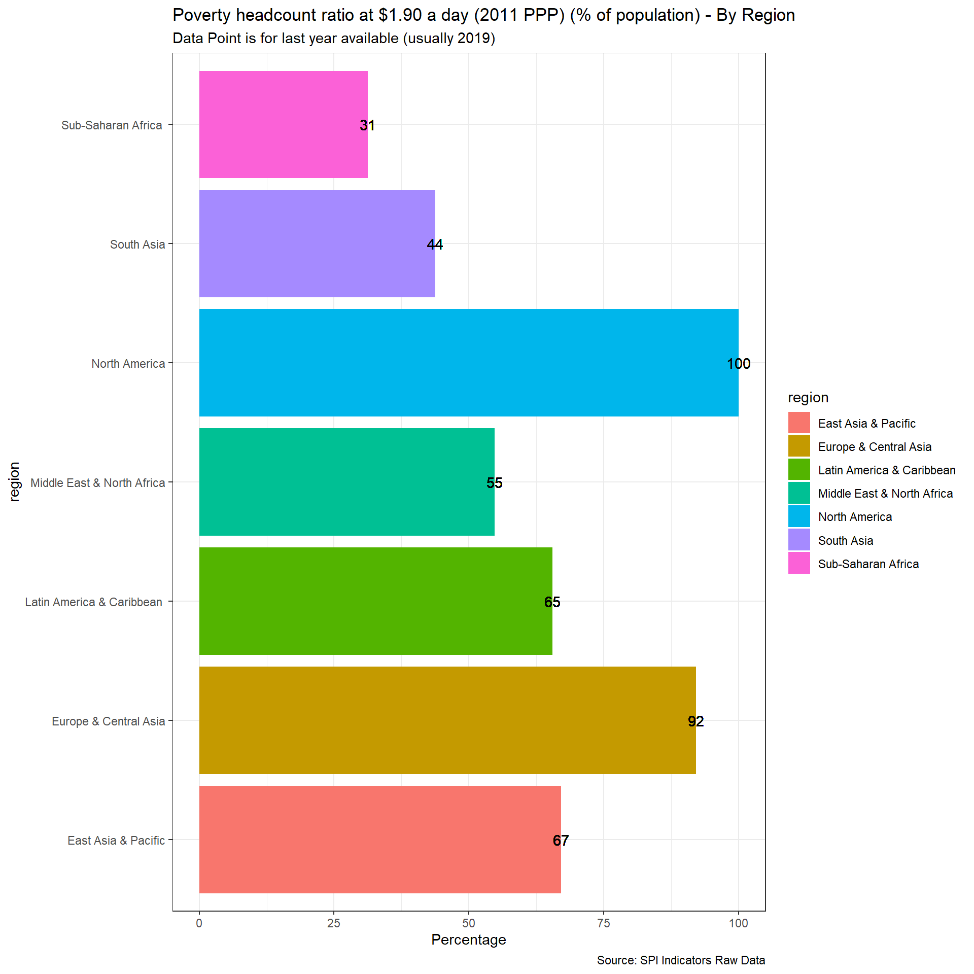
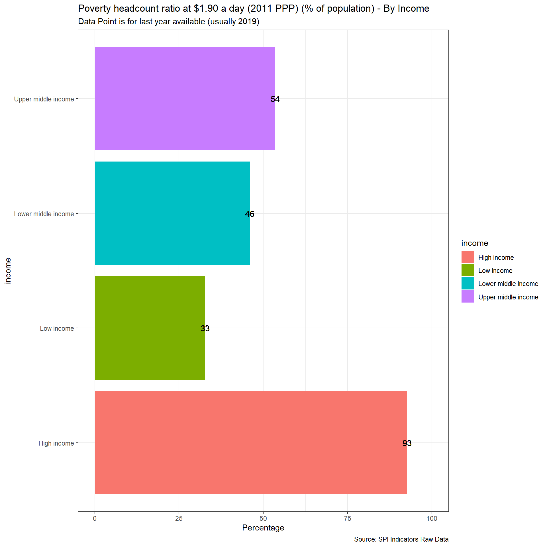
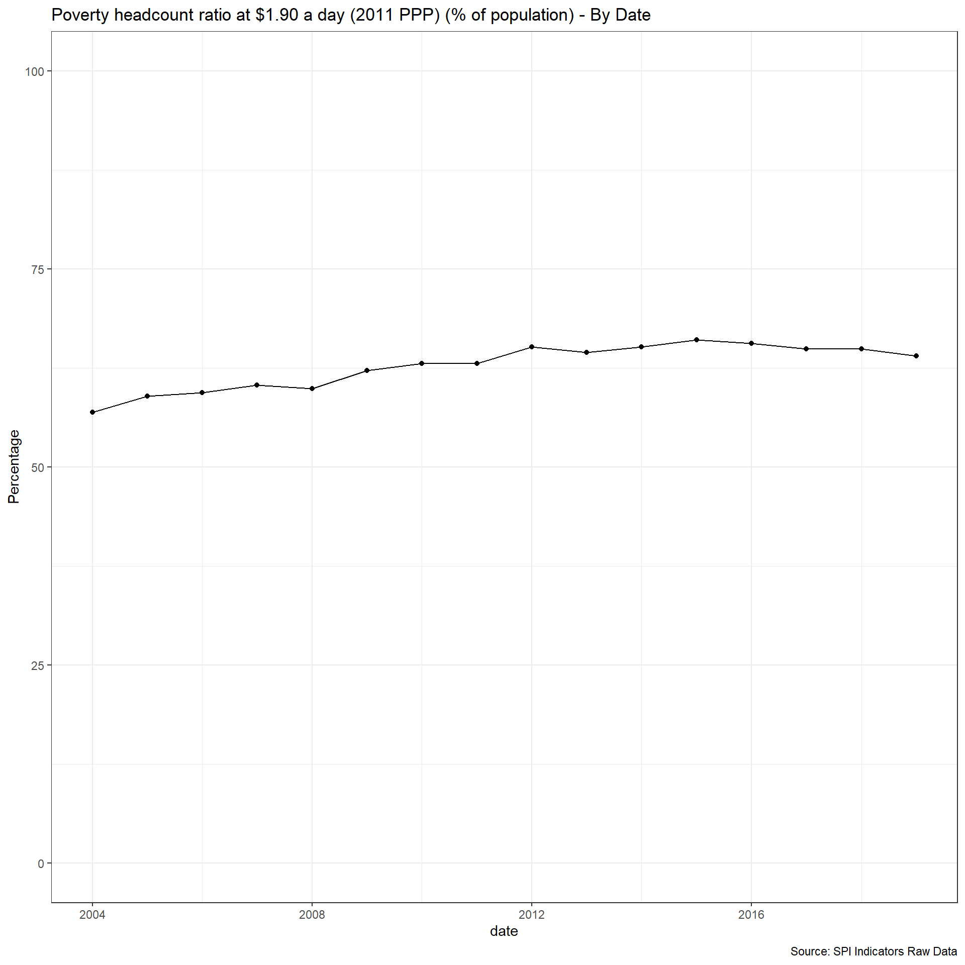
2.1.5.1 Poverty Comparability
The first measure examines whether comparable poverty estimates are produced by countries over time. The World Bank’s Povcalnet has introduced a comparability indicator for whether the country produces comparable poverty estimates over time. https://blogs.worldbank.org/opendata/apples-apples-povcalnet-introduces-new-comparability-indicator. This metadata has been compiled by the Country Poverty Economists in the World Bank’s Poverty and Equity Global Practice. From the Povcalnet team:
As countries frequently improve household surveys and measurement methodologies, strict comparability of poverty estimates over time is often limited. Strictly comparable poverty estimates within a country require a consistent production process, including the sampling frame, questionnaires, the methodological construction of the welfare aggregates and poverty lines, a consistent deflation of prices in time and space, among many other considerations. Thus, the assessment of comparability is country-dependent and relies on the knowledge of the Country Poverty Economist and Regional Poverty Teams of the Poverty Global Practice, as well as close dialogue with national data producers with intimate knowledge of the survey design and methodology. Within a country, we assume comparability of poverty estimates over time unless there is a known change to survey methodology, measurement or data structure. More details on the comparability metadata database can be found in Atamanov et al. (2019) (section 4). The database can be downloaded in csv.
The data will be pulled from the WDI and combined with metadata from the Povcalnet
Scoring is as follows:
Quality (1 points total):
1 Point. Comparable data lasting at least two years within past 5 years
0.5 Point. Comparable data lasting at least two years within past 10 years
0 Points. No comparable data within past 10 years
Note: Because poverty surveys are reported with a lag, we start measuring whether comparable poverty data is available two years prior. So for 2019, the window starts from 2017 to give countries time to prepare poverty estimates based on surveys.
library(povcalnetR)

#the code below is based on public released code by povcalnet team:
#https://github.com/worldbank/Global_Poverty_Blogs/blob/master/bg_povcalnet_comparability/R/comparability_breaks.R

## some contants
year_range <- 1990:2020
metadata_path <- "https://development-data-hub-s3-public.s3.amazonaws.com/ddhfiles/506801/povcalnet_comparability.csv"

## Load data ---------------------------------------------------------------

metadata <- read_csv(metadata_path)
cov_lkup <- c(3, 2, 1, 4)
names(cov_lkup) <- c("N", "U", "R", "A")

dat_lkup <- c(2,1)
names(dat_lkup) <- c("income","consumption")


pcn <- povcalnet()
pcn$coveragetype <- cov_lkup[pcn$coveragetype]
pcn$datatype <- dat_lkup[pcn$datatype]

df <- pcn %>%
  mutate(countrycode=as.character(countrycode)) %>%
  inner_join(metadata, by = c("countrycode", "year", "coveragetype", "datatype"))


#Now loop from 2016 and 2019, keeping just data inside last 5 years.
for (reference_year in 2004:2019) {

    #extend the window for more recent years.  For instance, 2019 surveys are reported with a lag, so give them two year grace period
  if (reference_year==2019) {
    rec_window=7
  } else if (reference_year==2018) {
    rec_window=6
  } else {
    rec_window=5
  }


  temp_5<-df %>%
        filter(coveragetype %in% c(3,4)) %>% #keep just nationally representative samples

        mutate(frequency=((reference_year-as.numeric(year))<=rec_window) & (reference_year>=as.numeric(year))) %>%
        filter(frequency==TRUE) %>%
        group_by(countrycode, comparability) %>% #for each country and comparability type, get number of comparable estimates
        summarise(SPI.D1.5.POV_5=n())  %>%
        ungroup() %>%
        group_by(countrycode) %>% #now get a total by country with the max number of comparable estimates
        summarise(SPI.D1.5.POV_5=max(SPI.D1.5.POV_5, na.rm=T)) %>%
        mutate(SPI.D1.5.POV_5=if_else(SPI.D1.5.POV_5>=2,1,0)) %>% #only give point if there is at least two observations that are comparable
        mutate(date=reference_year,
                 iso3c=countrycode) %>%
        left_join(country_metadata) %>%
        select( country,iso3c, date, starts_with('SPI.D1.5.POV'))

  temp_10<-df %>%
        filter(coveragetype %in% c(3,4)) %>% #keep just nationally representative samples
        mutate(frequency=((reference_year-as.numeric(year))<=12) & (reference_year>=as.numeric(year))) %>%
        filter(frequency==TRUE) %>%
        group_by(countrycode, comparability) %>% #for each country and comparability type, get number of comparable estimates
        summarise(SPI.D1.5.POV_10=n())  %>%
        ungroup() %>%
        group_by(countrycode) %>% #now get a total by country with the max number of comparable estimates
        summarise(SPI.D1.5.POV_10=max(SPI.D1.5.POV_10, na.rm=T)) %>%
        mutate(SPI.D1.5.POV_10=if_else(SPI.D1.5.POV_10>=2,1,0)) %>% #only give point if there is at least two observations that are comparable
        mutate(date=reference_year,
                 iso3c=countrycode) %>%
        left_join(country_metadata) %>%
        select( country,iso3c, date, starts_with('SPI.D1.5.POV'))

  temp <- temp_5 %>%
    left_join(temp_10) %>%
    mutate(SPI.D1.5.POV=case_when(
      SPI.D1.5.POV_5==1 ~ 1,
      SPI.D1.5.POV_10==1 ~ 0.5,
      TRUE ~ 0
    )) %>%
    select(-SPI.D1.5.POV_5,-SPI.D1.5.POV_10)

  assign(paste("D3.1.AKI",reference_year,sep="_"), temp)
}

#now append together and save
for (i in c(2004:2019)) {

  temp<-get(paste('D3.1.AKI_',i, sep=""))

  if (!exists('D3.1.AKI')) {
    D3.1.AKI<-temp
  } else {
    D3.1.AKI<-D3.1.AKI %>%
      bind_rows(temp) %>%
      arrange(-date, iso3c)
  }
}

#fix countries not included
D3.1.AKI<-D3.1.AKI %>%
  right_join(spi_df_empty) %>%
  mutate(SPI.D1.5.POV=if_else(lendingID=="LNX",1,SPI.D1.5.POV)) %>%#we give non-IDA/IBRD/blend countries credit for this, because they are not measured in database
  select(country, iso3c, date, SPI.D1.5.POV)
2.1.5.2 Mortality rate, under-5 (per 1,000 live births)
UN IGME makes all available source data on child mortality rates available with metadata on quality.
https://childmortality.org/data/
Source data can bedivided into data included in the estimation model and data excluded from the estimation model (note: data may be excluded for any one of several reasons including data quality or by rule—for example, indirect estimates from summary birth histories are not included when direct estimates from the full birth history from the same survey or census are available).
Countries are assessed for whether they can produce indicators over a five or ten year period that meet the thresholds set by UN IGME.
Quality (1 points total):
1 Point. Two indicators that met UN IGME standards within past 5 years
0.5 Point. Two indicators that met UN IGME standards within past 10 years
0 Points. No data that met UN IGME standards within past 10 years
Data was pulled on April 13, 2020.
Note: Because surveys are reported with a lag, we start measuring whether comparable poverty data is available two years prior. So for 2019, the window starts from 2017 to give countries time to prepare poverty estimates based on surveys.
#Read in data from UN Inter-agency Group for Child Mortality Estimation
D3.3.AKI.MORT <- read_csv(file=paste(raw_dir, '1.5_DUIO/UN IGME Child Mortality and Stillbirth Estimates.csv', sep="/")) %>%
as_tibble(.name_repair = 'universal') %>%
filter(Indicator=='Under-five mortality rate' & Sex=='Total') %>% #keep just observations for under 5 child mortality and for both sexes
filter(Observation.Status=='Included in IGME') %>% ## Also keep only surveys that met IGME criteria for inclusion as a nationally representative statistic
mutate(date=as.numeric(str_extract(Series.Year, "^.{4}")),
ind_date=as.numeric(str_extract(TIME_PERIOD, "^.{4}")),
country=Geographic.area,
D3.CHLD.MORT=OBS_VALUE)
#Now loop from 2016 and 2019, keeping just data inside last 5 years.
for (reference_year in 2004:2019) {
#extend the window for more recent years. For instance, 2019 surveys are reported with a lag, so give them two year grace period
if (reference_year==2019) {
rec_window=7
} else if (reference_year==2018) {
rec_window=6
} else {
rec_window=5
}
temp_5 <-D3.3.AKI.MORT %>%
mutate(frequency=(((reference_year-as.numeric(date))<=rec_window & (reference_year>=as.numeric(date))) | ((reference_year-as.numeric(ind_date))<=rec_window & (reference_year>=as.numeric(ind_date))))) %>% #whether to use the survey year or indicator report year depends on data source. for vital statistics sources need to use indicator reporting year, but for surveys use survey year
mutate(SPI.FREQ.D1.5.CHLD.MORT=if_else(frequency==TRUE,1,0)) %>% #create 0,1 variable for whether data point exists for country
group_by(country) %>%
summarise(SPI.FREQ.D1.5.CHLD.MORT=sum(SPI.FREQ.D1.5.CHLD.MORT, na.rm=T)) %>%
mutate(SPI.FREQ.D1.5.CHLD.MORT=case_when(
SPI.FREQ.D1.5.CHLD.MORT>=2 ~ 1,
TRUE ~ 0
)) %>%
mutate(SPI.D1.5.CHLD.MORT_5=SPI.FREQ.D1.5.CHLD.MORT) %>%
mutate(date=reference_year) %>%
select( country, date, starts_with('SPI.')) %>%
select(-SPI.FREQ.D1.5.CHLD.MORT)
temp_10 <-D3.3.AKI.MORT %>%
mutate(frequency=((reference_year-as.numeric(date))<=rec_window) & (reference_year>=as.numeric(date))) %>%
mutate(SPI.FREQ.D1.5.CHLD.MORT=if_else(frequency==TRUE,1,0)) %>% #create 0,1 variable for whether data point exists for country
group_by(country) %>%
summarise(SPI.FREQ.D1.5.CHLD.MORT=sum(SPI.FREQ.D1.5.CHLD.MORT, na.rm=T)) %>%
mutate(SPI.FREQ.D1.5.CHLD.MORT=case_when(
SPI.FREQ.D1.5.CHLD.MORT>=2 ~ 1,
TRUE ~ 0
)) %>%
mutate(SPI.D1.5.CHLD.MORT_10=SPI.FREQ.D1.5.CHLD.MORT) %>%
mutate(date=reference_year) %>%
select( country, date, starts_with('SPI.')) %>%
select(-SPI.FREQ.D1.5.CHLD.MORT)
temp <- temp_5 %>%
left_join(temp_10) %>%
mutate(SPI.D1.5.CHLD.MORT=case_when(
SPI.D1.5.CHLD.MORT_5==1 ~ 1,
SPI.D1.5.CHLD.MORT_10==1 ~ 0.5,
TRUE ~ 0
)) %>%
select(-SPI.D1.5.CHLD.MORT_5,-SPI.D1.5.CHLD.MORT_10)
assign(paste("D3.3.AKI",reference_year,sep="_"), temp)
}
#now append together and save
for (i in c(2004:2019)) {
temp<-get(paste('D3.3.AKI_',i, sep=""))
if (!exists('D3.3.AKI')) {
D3.3.AKI<-temp
} else {
D3.3.AKI<-D3.3.AKI %>%
bind_rows(temp) %>%
arrange(-date, country)
}
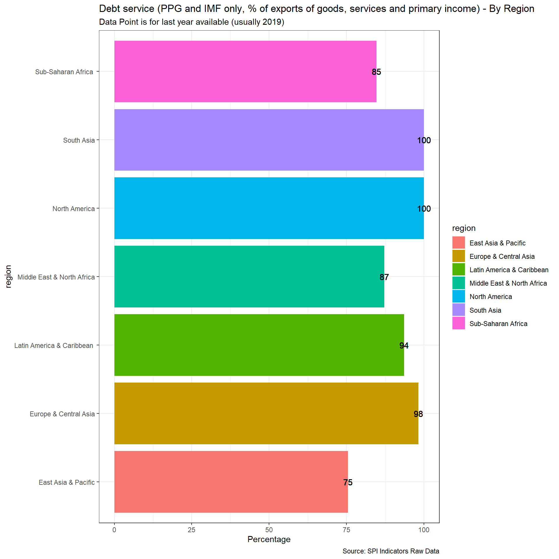
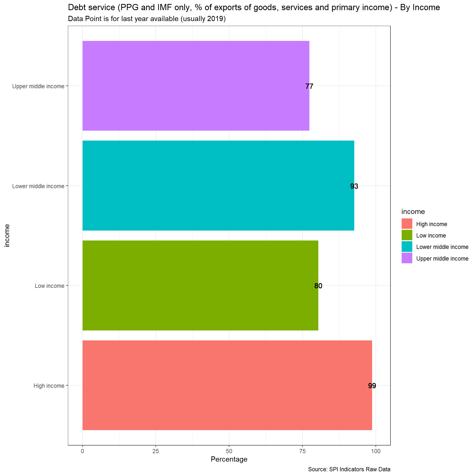
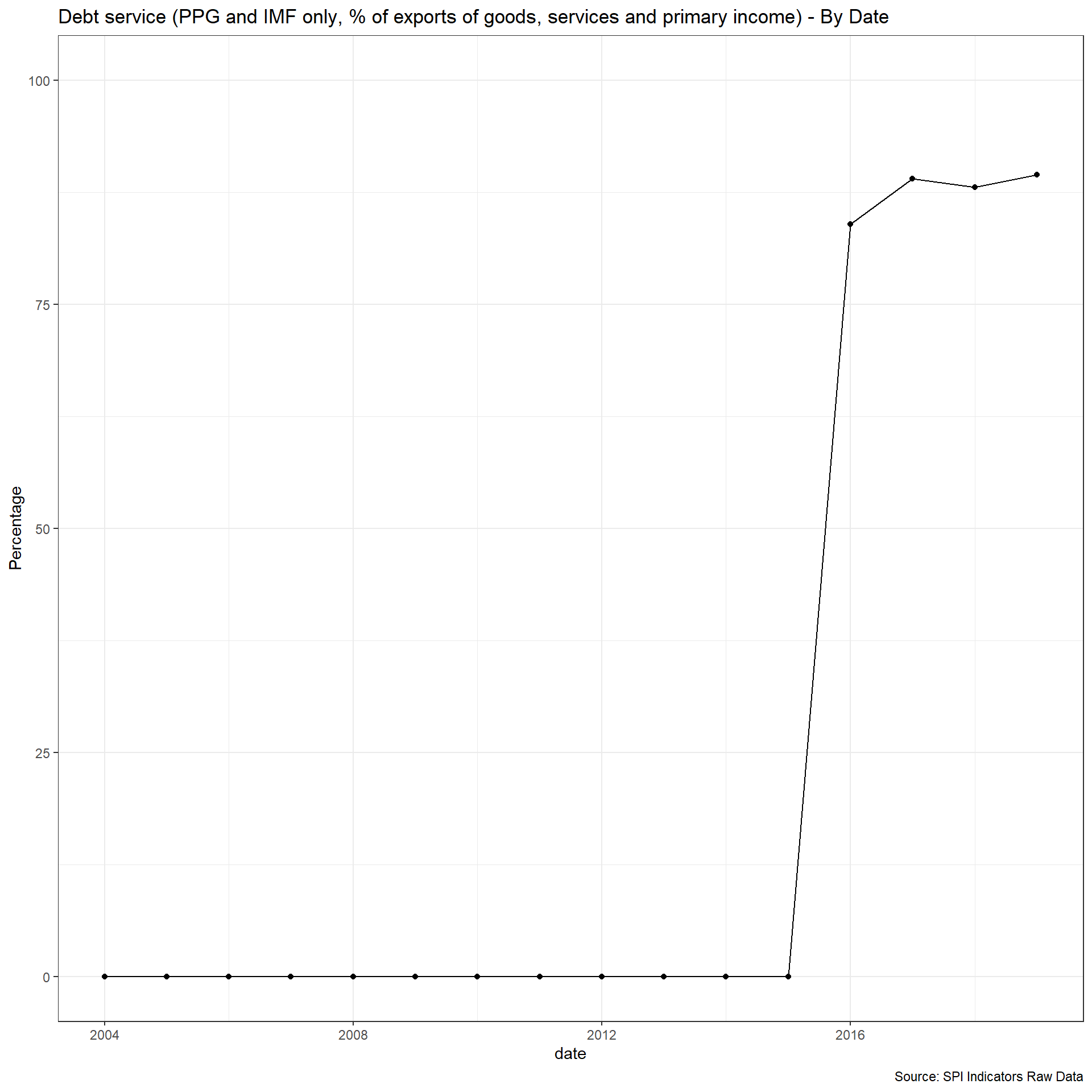
}2.1.5.3 Debt service (PPG and IMF only, % of exports of goods, services and primary income)
For this indicator, Debt service (PPG and IMF only, % of exports of goods, services and primary income), we will pull data from the WDI but modify the scoring using the WDI metadata on whether the external debt data is actual, estimated, or preliminary. The status “as reported (actual)” indicates that the country was fully current in its reporting under the DRS and that World Bank staff are satisfied that the reported data give an adequate and fair representation of the country’s total public debt. “Preliminary” data are based on reported or collected information, but because of incompleteness or other reasons, an element of staff estimation is included. “Estimated” data indicate that countries are not current in their reporting and that a significant element of staff estimation has been necessary for producing the data tables.
Scoring is as follows:
Quality:
1 Points. Actual value 0.67 Points. Preliminary value 0.33 Points. Estimated value 0 Points. No value
#reshape metaadata file
D3.15.AKI <- WDI_metadata %>%
transmute(iso3c=if_else(is.na(Country.Code), Code, Country.Code),
date=date,
External_debt_Reporting=External.debt.Reporting.status,
Income.Group=Income.Group) %>%
mutate(SPI.D1.5.DT.TDS.DPPF.XP.ZS= case_when(
External_debt_Reporting=='Actual' ~ 1,
External_debt_Reporting=='Preliminary' ~ 0.67,
External_debt_Reporting=='Estimate' ~ 0.33,
TRUE ~ 0
)) %>%
mutate(SPI.D1.5.DT.TDS.DPPF.XP.ZS=if_else(((Income.Group=="High income" | iso3c %in% c("WBG", "PSE")) & is.na(External_debt_Reporting)),1,SPI.D1.5.DT.TDS.DPPF.XP.ZS)) %>% #fix an issue where high income countries are not judged on their debt reporting. Also give credit to West Bank and Gaza as they are not an IMF country
ungroup() %>%
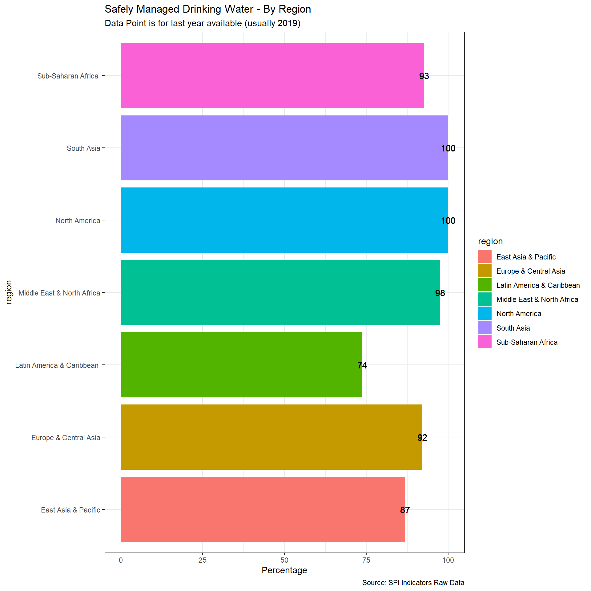
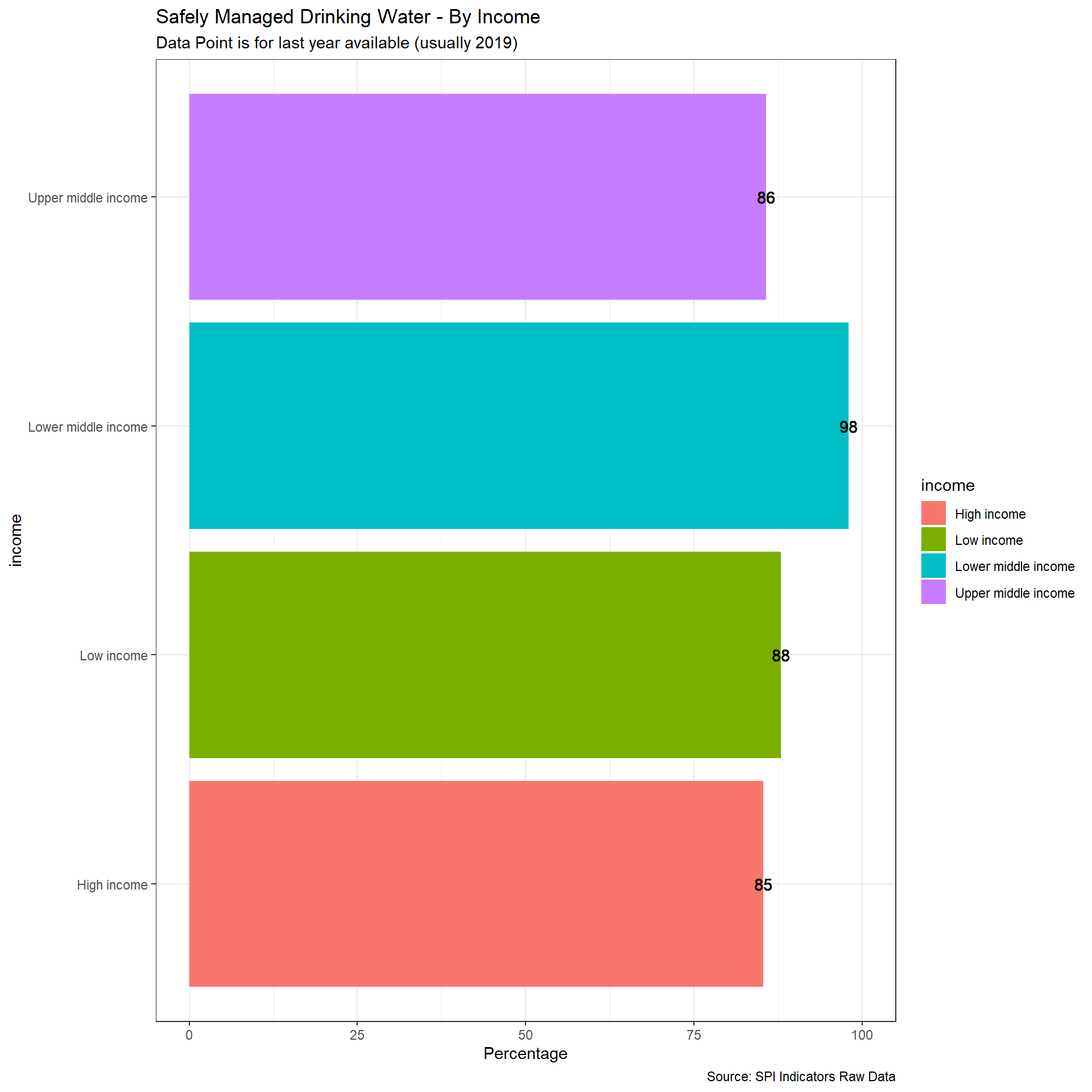
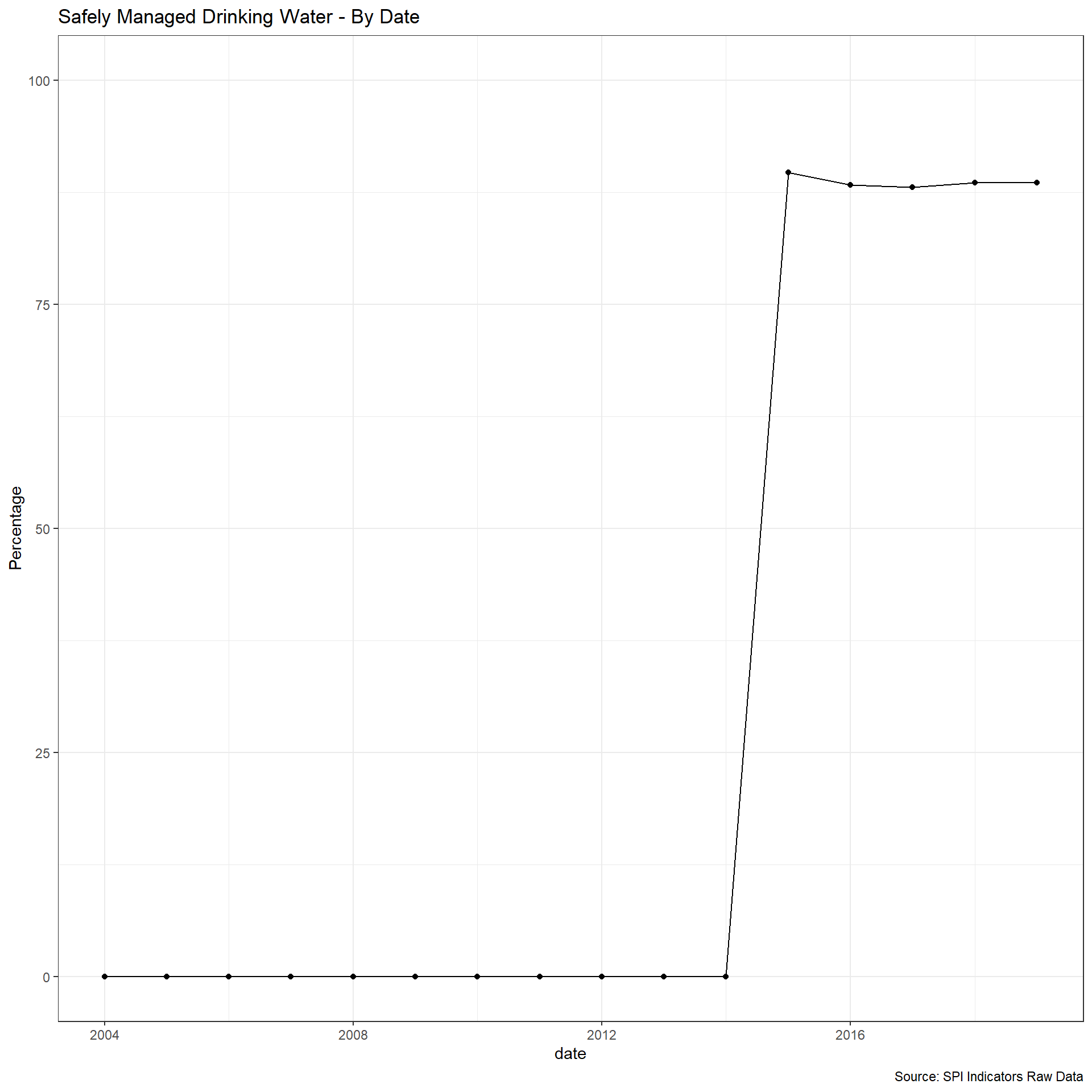
select(iso3c, date, contains('SPI.D1.5.DT.TDS.DPPF.XP.ZS')) 2.1.5.4 Safely Managed Water
The WHO/UNCIECF JMP has estimated the safely managed water access by a simple linear regression based on the following data sources: Nationally representative household surveys (e.g. DHS, MICS) ; Population and housing censuses; Administrative data (such as regulatory agencies); Service provider data. JMP has provided the country files that include the original data sources.
From the methodology: https://washdata.org/sites/default/files/JMP%20methodology-Apr-2018-5.pdf:
The indicator for SDG 6.1, safely managed drinking water services are defined as use of an improved drinking water source which is accessible on premises, available when needed and free from contamination. To make an estimate of safely managed services, information on the use of improved drinking water sources is combined with information on the accessibility, availability and quality of drinking water. Estimates are based on the minimum value of these criteria or, where estimates are available for both rural and urban, a population weighted average of the two. The JMP reports estimates for safely managed drinking water provided information is available for at least 50 per cent of the population on quality of drinking water and either accessibility or availability.
We take therefore useable data if it appears within an 8 year window of the reference date. Scoring:
- 1 Point. At least two estimates, with breakdowns for urban/rural areas, within an 8 year window
- 0.5 Points. At least two estimates, but not an urban/rural breakdown, within an 8 year window
- 0 Points. Otherwise
#read in saved data
safely_managed_raw_df <- read_csv(file=paste(raw_dir, '1.5_DUIO/Safely_Managed_Water_data.csv', sep="/"))
#score the data
#function to calculate 10 year window
window_fun <- function(date_start, date_end) {
temp <- safely_managed_raw_df %>%
filter(between(year,date_start,date_end) ) %>%
group_by(iso3c, geo) %>%
summarise(data_quality=sum(data_quality, na.rm=T)) %>% #average over 10 years
pivot_wider(
names_from = 'geo',
values_from = 'data_quality'
) %>%
mutate(
SPI.D1.5.SAFE.MAN.WATER=case_when(
(Rural>=2 & Urban>=2) ~ 1, #urban rural breakdown gets 1 point
(Rural>=2 | Urban>=2 | National>=2) ~ 0.5, #partial data at at least one geography gets 0.5
TRUE ~ 0
)
) %>%
select(iso3c, SPI.D1.5.SAFE.MAN.WATER) %>%
mutate(date=date_end)
}
####
## 8 Year window
####
#create this database for each year from 2004 to 2019 using a 8 year window
for (i in c(2015:2019)) {
end=i
#extend the window for more recent years. For instance, 2019 surveys are reported with a lag, so give them two year grace period
if (end==2019) {
start=i-9
} else if (end==2018) {
start=i-8
} else {
start=i-7
}
temp_df <- window_fun(start,end)
assign(paste('safe_managed_',end, sep=""), temp_df)
}
if (exists('safe_managed_df')) {
rm('safe_managed_df')
}
#now append together and save
for (i in c(2015:2019)) {
temp<-get(paste('safe_managed_',i, sep=""))
if (!exists('safe_managed_df')) {
safe_managed_df<-temp
} else {
safe_managed_df<-safe_managed_df %>%
bind_rows(temp) %>%
arrange(-date, iso3c)
}
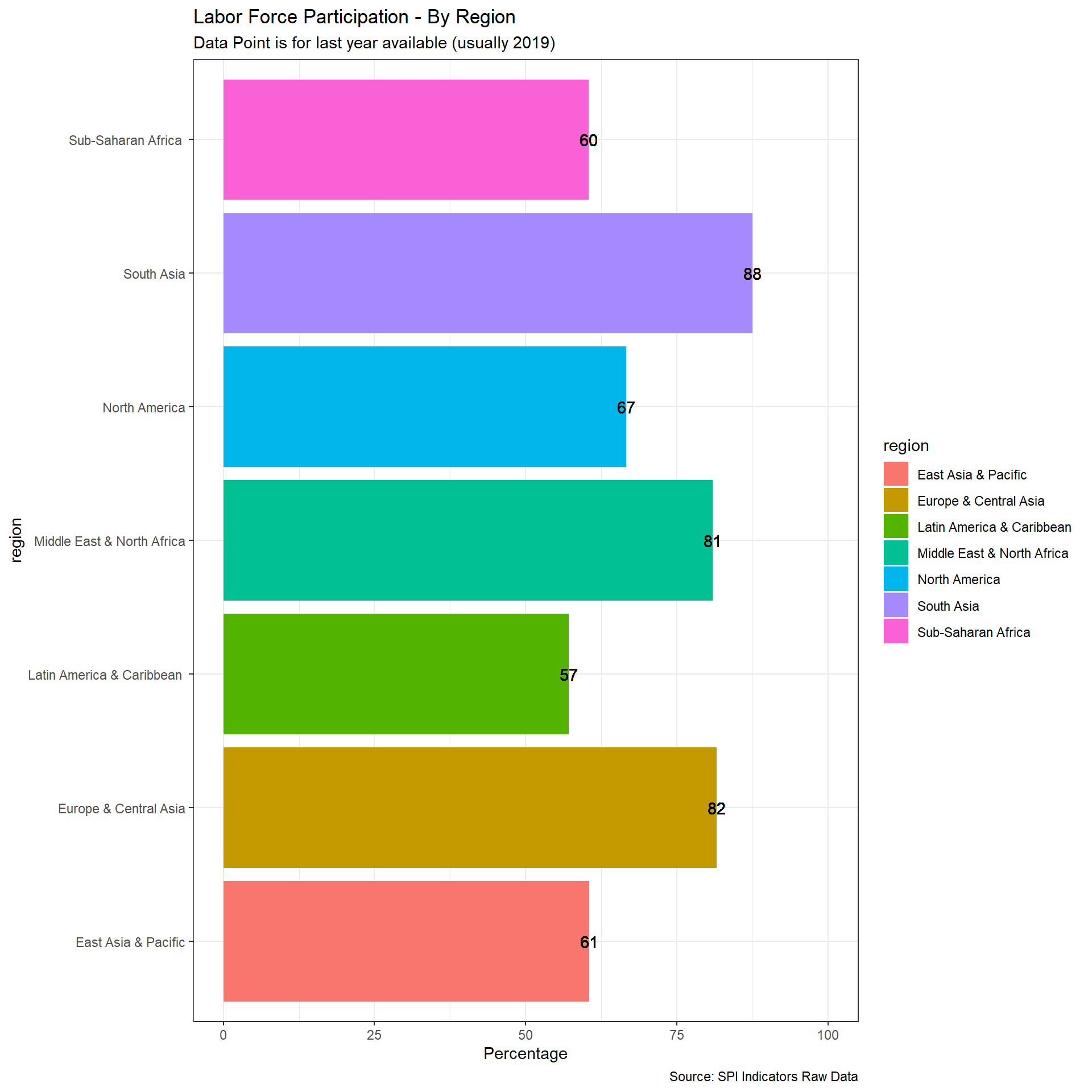
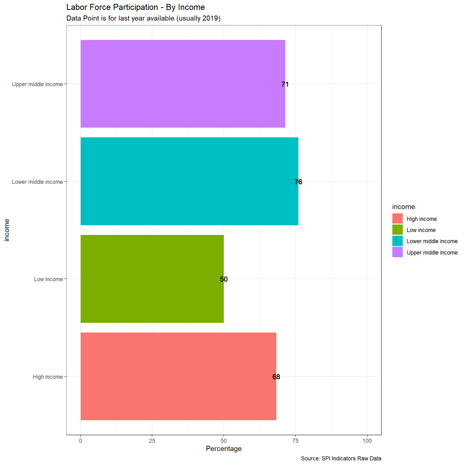
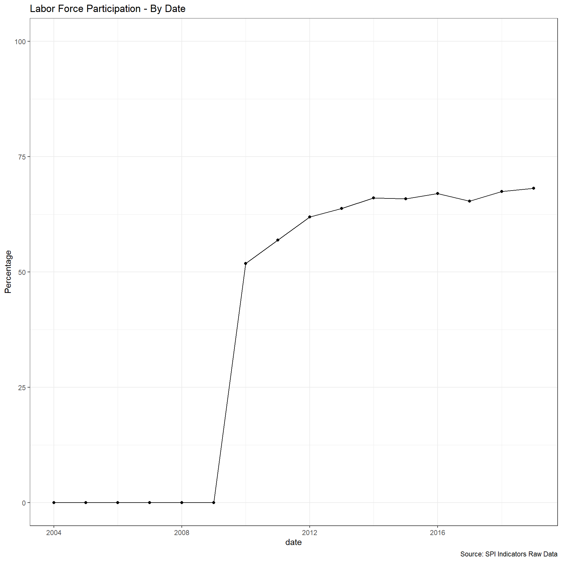
}2.1.5.5 Labor Force Statistics
In this indicator, we compare estimated labor force participation data compared to data submitted to the ILO based on national data. ILOSTAT is the source of both datasets. Countries are given full points if an indicator is produced by a national government based on a labor force survey and if that estimate is within 10 percentage points of the ILO estimated value. If either of those two components are missing, but one is available, then the country gets 0.5 points. O points otherwise.
The ILO modelled estimates series provides a complete set of internationally comparable labour statistics, including both nationally-reported observations and imputed data for countries with missing data. The imputations are produced through a series of econometric models maintained by the ILO. The purpose of estimating labour market indicators for countries with missing data is to obtain a balanced panel data set so that, every year, regional and global aggregates with consistent country coverage can be computed. These allow the ILO to analyse global and regional estimates of key labour market indicators and related trends. Moreover, the resulting country-level data, combining both reported and imputed observations, constitute a unique, internationally comparable data set on labour market indicators.
From the ILO methodological note (https://www.ilo.org/ilostat-files/Documents/TEM.pdf), ILO has the following preferences for data with Labor force surveys coming first:
With regard to the first criterion, in order for labour market data to be included in a particular model, they must be derived from a labour force survey, a household survey or, more rarely, a population census. National labour force surveys are generally similar across countries and present the highest data quality. Hence, the data derived from such surveys are more readily comparable than data obtained from other sources. Strict preference is therefore given to labour force survey-based data in the selection process. However, many developing countries, which lack the resources to carry out a labour force survey, do report labour market information on the basis of other types of household surveys or population censuses. Consequently, because of the need to balance the competing goals of data comparability and data coverage, some (non-labour force survey) household survey data and, more rarely, population census-based data are included in the models.
Scoring:
1 Point. Country has a labor force survey based estimate in past 5 years of labor force participation broken down by total, male, and female & estimated value from ILO is within 10 percentage points of value reported by national government.
0.5 Point. Country has labor force survey or is within 10 points of ILO, but not both
0 Points. Otherwise
#read in ILO reference areas
ilo_ref_area <- read_csv(file= paste0(raw_dir,"/metadata/ILO_reference_area.csv")) %>%
  transmute(iso3c=ref_area,
            country=ref_area.label)

#read in the ILO data downloaded on November 24, 2020
lfp_estimated <- read_excel(path = paste0(raw_dir,"/1.5_DUIO/ILO_lfp_country_estimated.xlsx"),
                            skip=5) %>%
  as_tibble(.name_repair = 'universal') %>%
  mutate(country=case_when(
    Reference.area=="Gambia" ~ "Gambia, The",
    TRUE ~ Reference.area
    ),
    date=Time,
    estimated_value=Total) %>%
    left_join(ilo_ref_area) %>%
  select(iso3c, date, Sex, estimated_value )

#reported data by countries
lfp_reported <- read_excel(path = paste0(raw_dir,"/1.5_DUIO/ILO_lfp_country_reported.xlsx"),
                           skip=5)%>%
  as_tibble(.name_repair = 'universal') %>%
  mutate(country=case_when(
    Reference.area=="Gambia" ~ "Gambia, The",
    TRUE ~ Reference.area
    ),
    date=Time,
    reported_value=..15.) %>%
    left_join(ilo_ref_area) %>%
  select(iso3c, date, Source.type, Sex, reported_value )

#merge the two together
lfp_data <- lfp_reported %>%
  left_join(lfp_estimated) %>%
  mutate(estimate_diff=reported_value-estimated_value,
         lfs_source=(Source.type=="Labour force survey")) %>%
  filter(iso3c %in% country_metadata$iso3c)


#score the data

#function to calculate 10 year window
ilo_fun <- function(date_start, date_end) {
  temp <- lfp_data %>%
    filter(between(date,date_start,date_end) ) %>%
    group_by(iso3c) %>%
    summarise(SPI.D1.5.LFP.ACC=as.numeric(mean(estimate_diff, na.rm=T)<=10),
              SPI.D1.5.LFP.SOURCE=max(lfs_source, na.rm=T),
              SPI.D1.5.LFP=(SPI.D1.5.LFP.ACC+SPI.D1.5.LFP.SOURCE)/2) %>%
    select(iso3c, SPI.D1.5.LFP) %>%
    mutate(date=date_end)

}
####
## 5 Year window
####
#create this database for each year from 2004 to 2019 using a 10 year window


for (i in c(2010:2019)) {

  end=i

    #extend the window for more recent years.  For instance, 2019 surveys are reported with a lag, so give them two year grace period
  if (end==2019) {
    start=i-6
  } else if (end==2018) {
    start=i-5
  } else {
    start=i-4
  }

  temp_df <- ilo_fun(start,end)
  assign(paste('lfp_data_',end, sep=""), temp_df)
}

if (exists('lfp_data_df')) {
  rm('lfp_data_df')
}
#now append together and save
for (i in c(2010:2019)) {

  temp<-get(paste('lfp_data_',i, sep=""))

  if (!exists('lfp_data_df')) {
    lfp_data_df<-temp
  } else {
    lfp_data_df<-lfp_data_df %>%
      bind_rows(temp) %>%
      arrange(-date, iso3c)
  }
}
## [1] "SPI.D1.5.POV"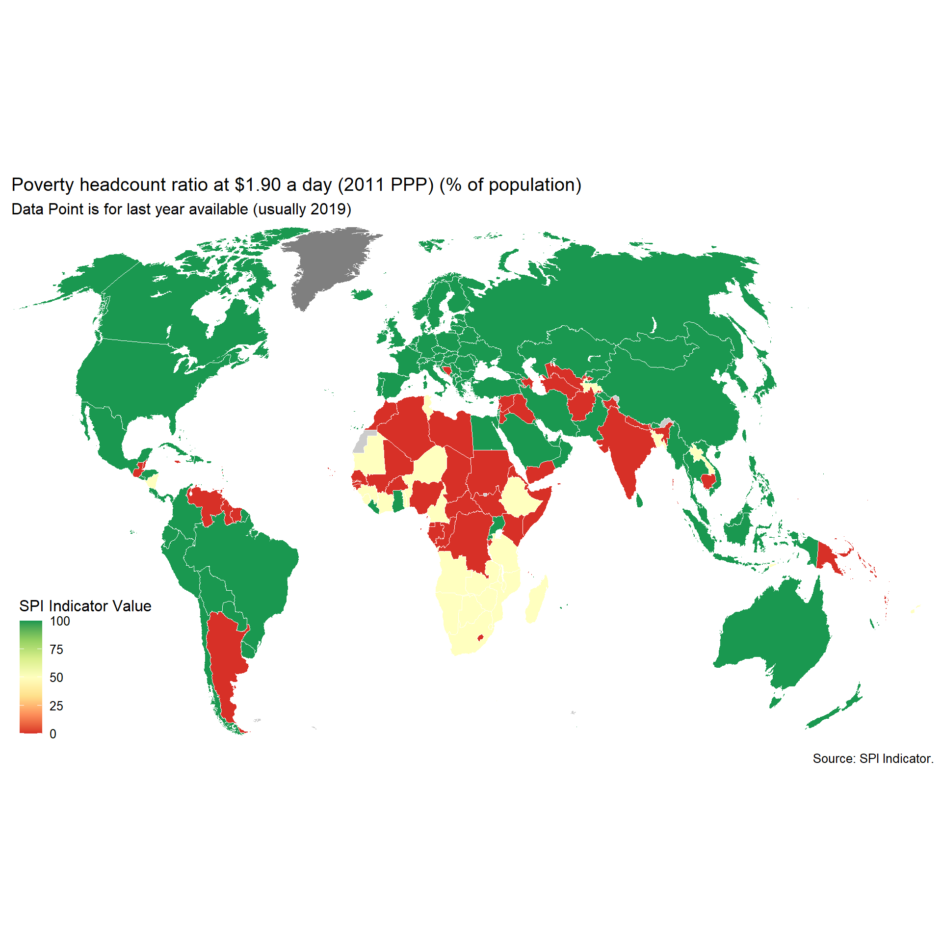
## [1] "SPI.D1.5.CHLD.MORT"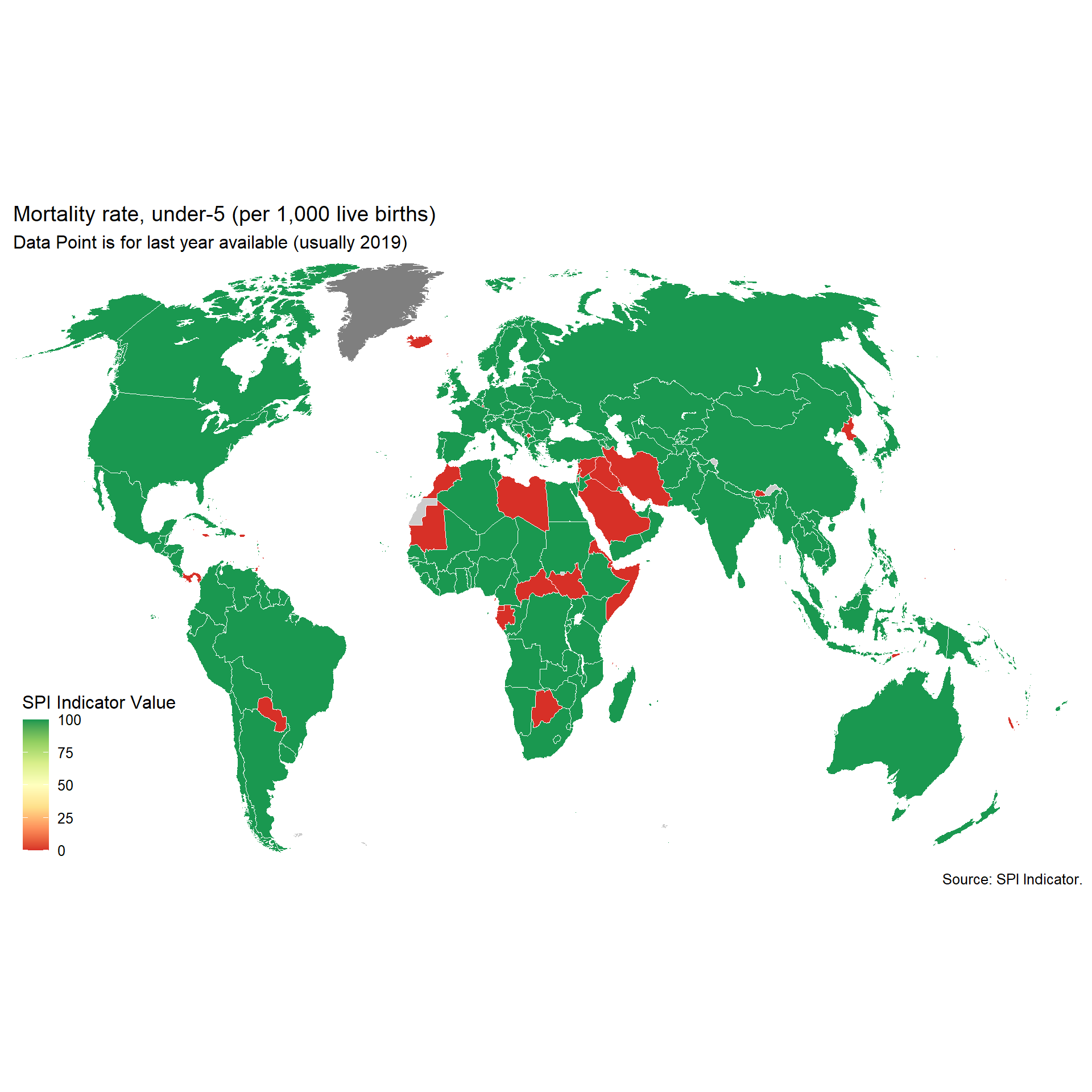
## [1] "SPI.D1.5.DT.TDS.DPPF.XP.ZS"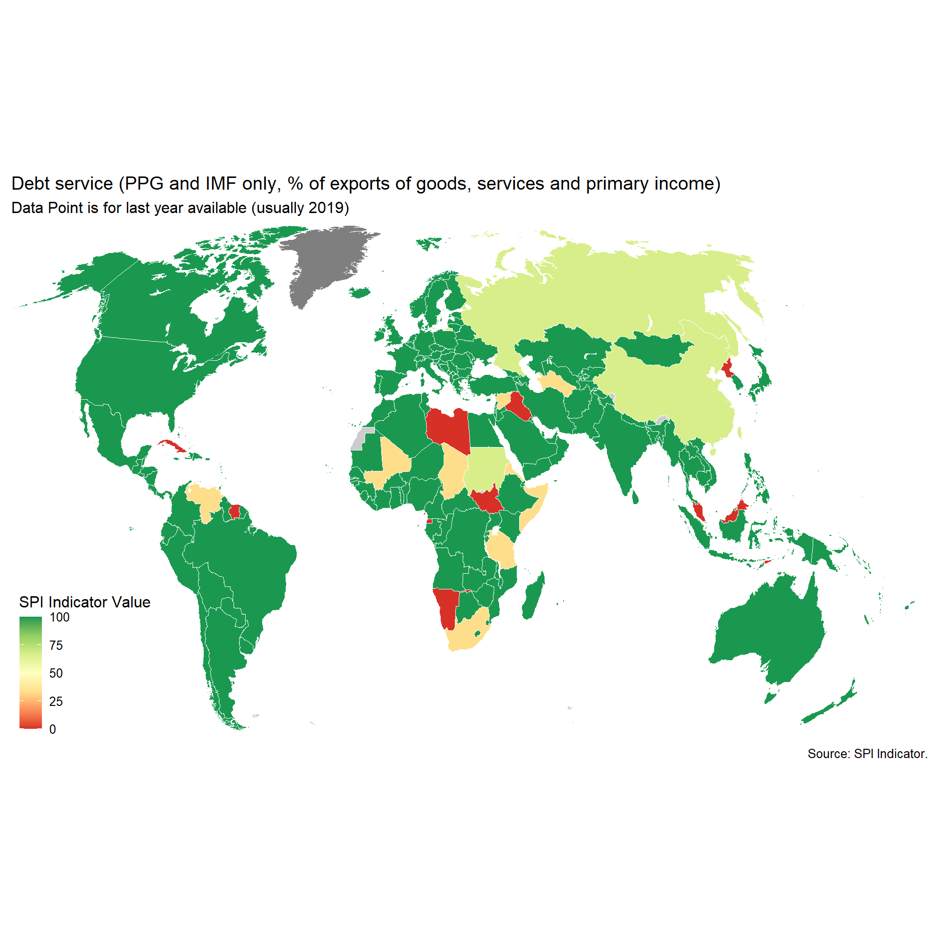
## [1] "SPI.D1.5.SAFE.MAN.WATER"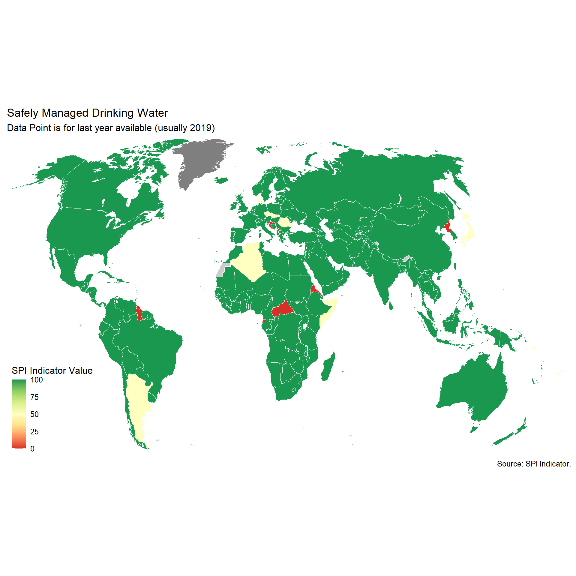
## [1] "SPI.D1.5.LFP"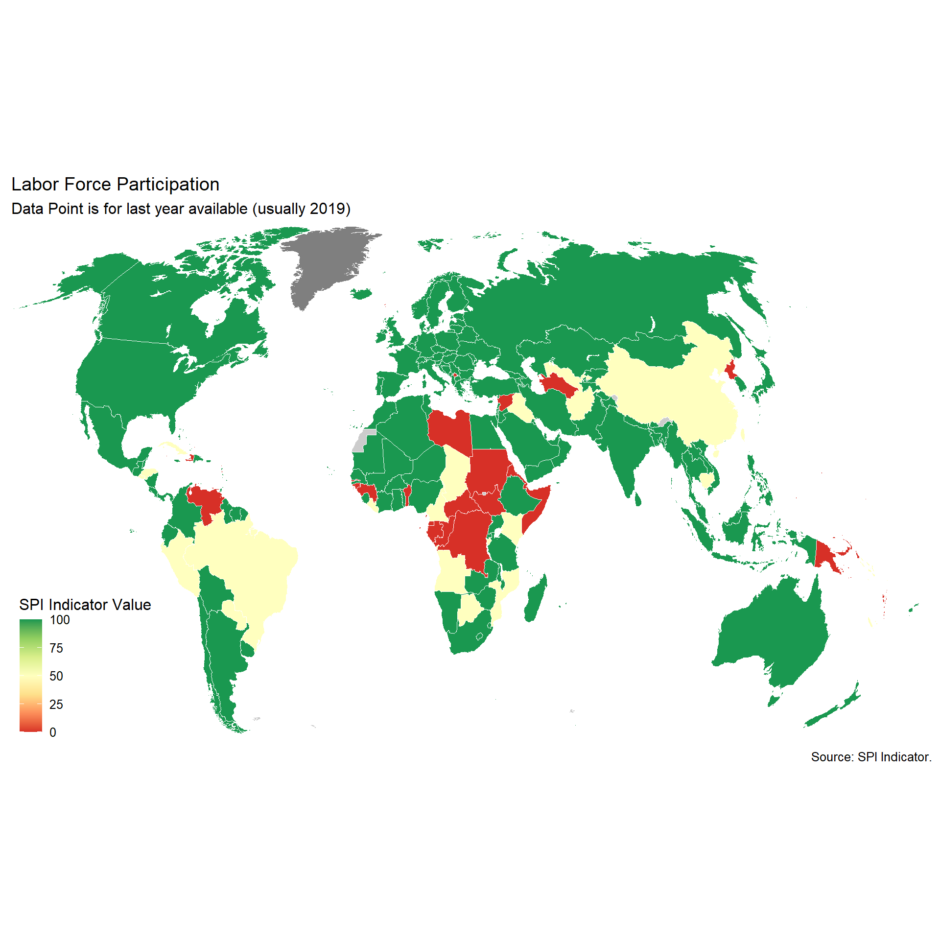
2.2 Data Services
Cleaning for Data Services Indicators. Data Services (4 Indicators):
- 2.1_DSDR - Indicator 2.1: Data releases
- 2.2_DSOA - Indicator 2.2: Online access
- 2.3_DSAS - Indicator 2.3: Advisory/ Analytical Services
- 2.4_DSDS - Indicator 2.4: Data services
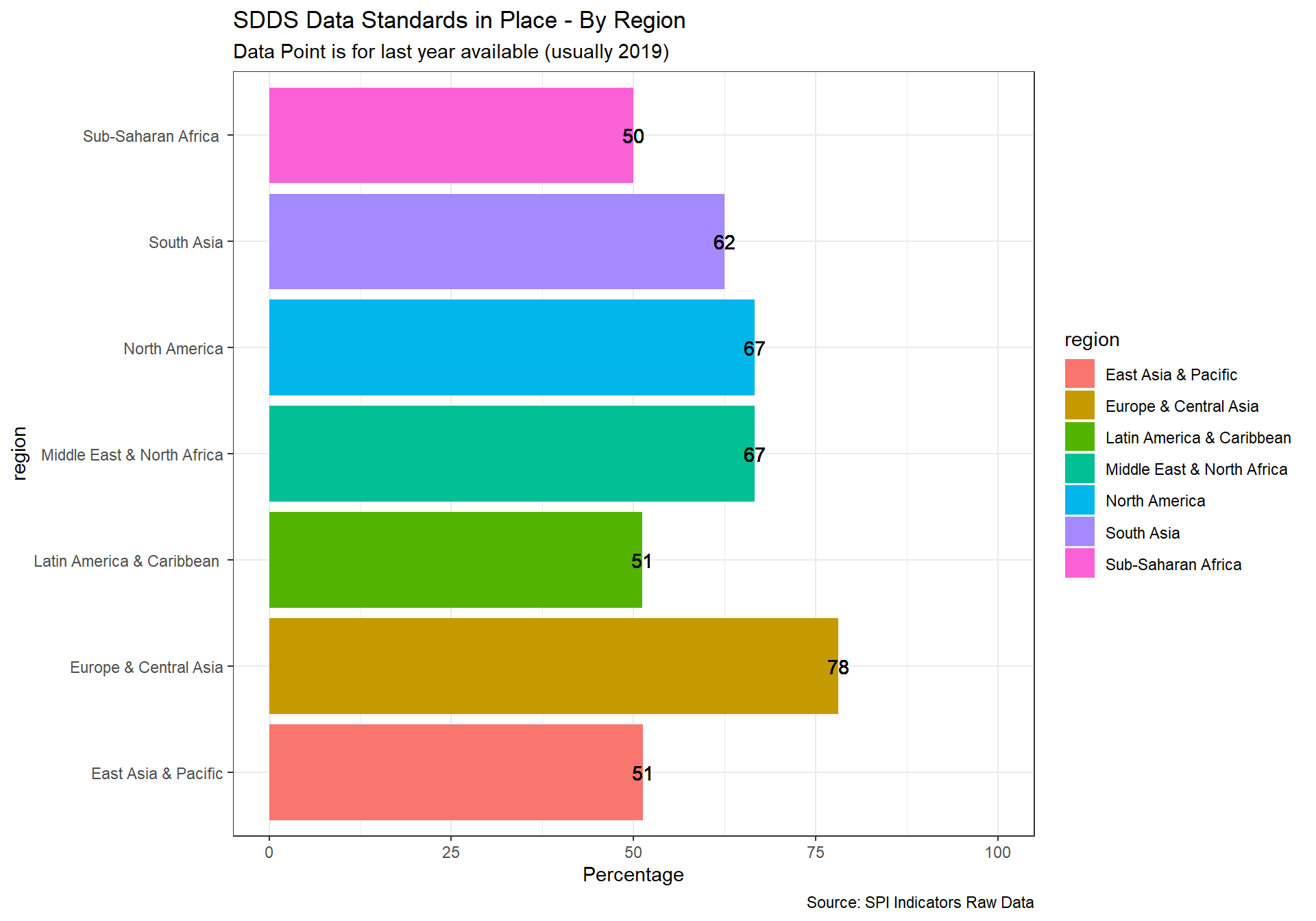
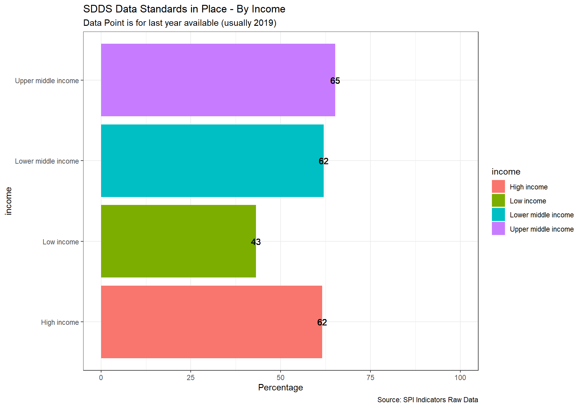
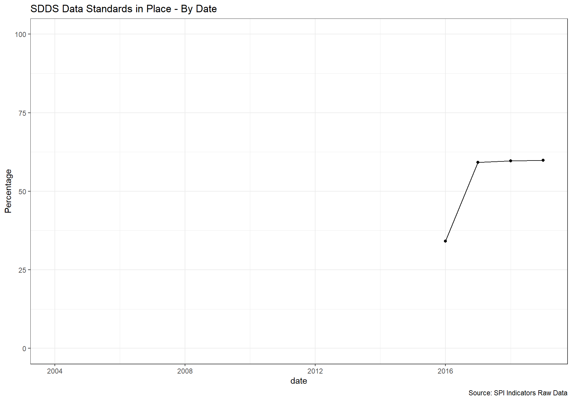
2.2.1 Indicator 2.1: Data Releases
Data Dissemination Standard (SDDS) and electronic General Data Dissemination Standard (e-GDDS) were established by the International Monetary Fund (IMF) for member countries that have or that might seek access to international capital markets, to guide them in providing their economic and financial data to the public. Although subscription is voluntary, the subscribing member needs to be committed to observing the standard and provide information about its data and data dissemination practices (metadata). The metadata are posted on the IMF’s SDDS and e-GDDS websites.
1 Point. Subscribing to IMF SDDS+ or SDDS standards 0.5 Points. Subscribing to IMF e-GDDS standards 0 Points. Otherwise
Request_metadata <- GET(url = "http://api.worldbank.org/v2/country/all/indicator/5.21.01.01.sdds?format=json&date=2004:2015&per_page=5000")
Response_metadata <- content(Request_metadata, as = "text", encoding = "UTF-8")

## Parse the JSON content and convert it to a data frame.
D2.1_DSDR_sci <- jsonlite::fromJSON(Response_metadata, flatten = TRUE) %>%
  data.frame() %>%
  transmute(
    iso3c=countryiso3code,
    country=country.value,
    date=as.numeric(date),
    SDDS=if_else(is.na(value),0,as.numeric(value))
  ) %>%
  left_join(spi_df_empty) %>% #add on country metadata
  filter(!is.na(income)) %>%
  select(iso3c, country, date, SDDS  )


#read in metadata file.

#pull data for several of the standards from WDI metadata

df <- WDI_metadata

## Manipulate and clean final data
df <- df %>%
  filter(!is.na(Income.Group))  #keep just countries (drop aggregations)


D2.1_DSDR <- df %>%
  mutate(iso3c=if_else(is.na(Country.Code), Code, Country.Code),
         country=Table.Name) %>%
  select(c('iso3c', 'country', 'date',  'IMF.data.dissemination.standard')  ) %>%
  mutate(IDDS=IMF.data.dissemination.standard) %>%
  mutate(SPI.D2.1.GDDS=case_when(
    IDDS=="Special Data Dissemination Standard Plus (SDDS+)" | IDDS=="Special Data Dissemination Standard (SDDS)"~ 1,
    IDDS=="Enhanced General Data Dissemination System (e-GDDS)"~ 0.5,
    TRUE ~ 0 ),
    SDDS=case_when(
     IDDS=="Special Data Dissemination Standard (SDDS)"~ 1,
    TRUE ~ 0 ))  %>%
  bind_rows(D2.1_DSDR_sci) %>%
  rename(RAW.D2.1.GDDS=IDDS) %>%
  select(iso3c,  date, RAW.D2.1.GDDS, SPI.D2.1.GDDS  ) %>%
  left_join(country_metadata)

D2.1_DSDR_map <- D2.1_DSDR


spi_mapper('D2.1_DSDR_map', 'SPI.D2.1.GDDS', 'SDDS Data Standards in Place' )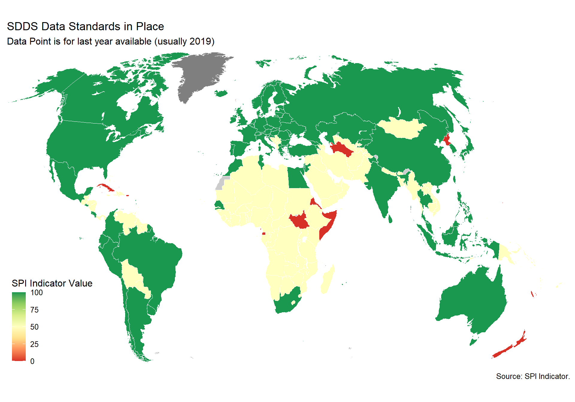
#add to spi databases
spi_df <- spi_df %>%
  left_join(D2.1_DSDR)
2.2.2 Indicator 2.2: Online access
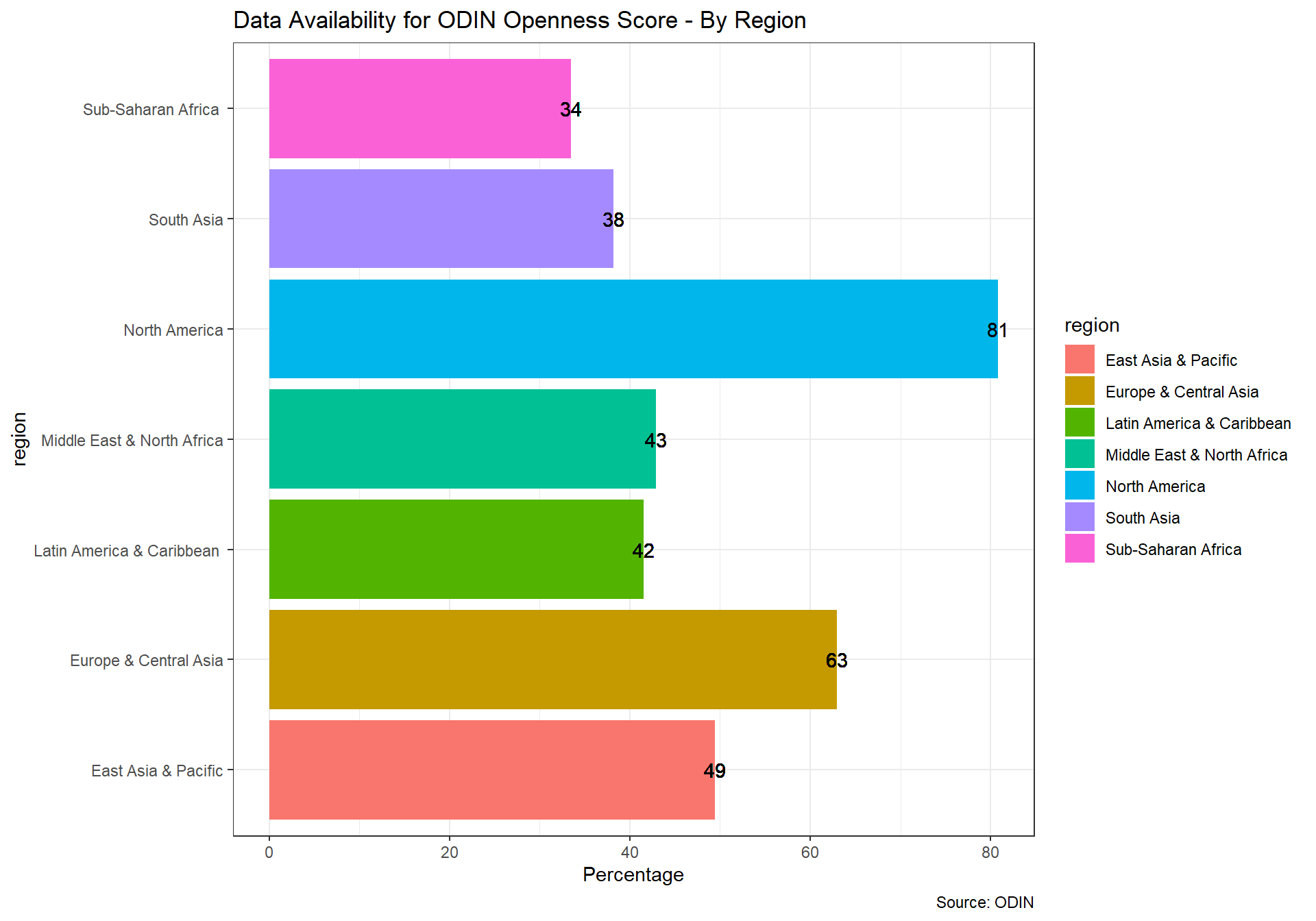
This indicator measures the richness and openness of online access.
2.2.2.1 Source
Our source for this indicator is Open Data Watch. Data was last accessed on December 17, 2020. From Open Data watch:
The Open Data Inventory (ODIN) assesses the coverage and openness of official statistics to help identify gaps, promote open data policies, improve access, and encourage dialogue between national statistical offices (NSOs) and data users. ODIN 2018/19 includes 178 countries, including most all OECD countries. Two-year comparisons are for all countries with two years of data between 2015-2017. Scores can be compared across topics and countries.
We use the Openness score from ODIN for this measure. The score ranges from 0-100. It contains scores along five dimensions:
- Machine Readability
- Non-Proprietary format
- Download Options
- Metadata Available
- Terms of Use
A description for each of these five dimensions is below:
2.2.2.1.1 Machine Readability
Openness element 1 measures whether data are available in a machine readable format such as XLS, XLSX, CSV, and JSON. Machine-readable file formats allow users to easily process data using a computer. When data are made available in formats that are not machine readable, users cannot easily access and modify the data, which severely restricts the scope of the data’s use. In many cases PDF versions of datasets within reports can be useful to users, as the text in conjunction with the tables gives context and explanation to the figures which helps less technical users understand the data. Because of this, ODIN assessments do not penalize countries for making datasets available in PDF or other non-machine readable formats, unless these formats are the only option for exporting data. Scores are not penalized for having identical datasets in both machine readable and non-readable formats. Compression formats do not affect machine readability scores, only non-proprietary scores (see next page). Scores are given by data category, not indicator.
2.2.2.1.2 Non-Proprietary format
For the elements of data openness, scoring is calculated independent of the data coverage. If data files are compressed in RAR format (which is proprietary), data for that indicator should be considered proprietary even if the enclosing files are in a non-proprietary format. Files compressed in ZIP format are not affected.
2.2.2.1.3 Download Options
Openness element 3 measures whether data are available with three different download options: bulk download, API, and user-select options. A bulk download is defined at the indicator level as: The ability to download all data recorded in ODIN for a particular indicator (all years, disaggregations, and subnational data) in one file, or multiple files that can be downloaded simultaneously. Bulk downloads are a key component of the Open Definition, which requires data to be “provided as a whole . . . and downloadable via the internet.” User-selectable download options are defined as: Users must be able to select an indicator and at least one other dimension to create a download or table. These dimensions could include time periods, geographic disaggregations, or other recommended disaggregations. An option to choose the file export format is not enough. API stands for Application Programming Interface. Ideally, APIs should be clearly displayed on the website. ODIN assumes APIs are available for the NSOs entire data collection used in ODIN, unless clearly stated. ODIN assessors do not register for use or test API functionality. For more information on APIs, see this guide. Scores are given by data category, not indicator.
2.2.2.1.4 Metadata Available
Openness element 4 measures whether metadata are made available. Scores are given by data category, not indicator. Metadata are defined at the indicator level as information about how the data are defined/calculated and collected. ODIN classifies metadata into three categories: (1) Not Available, (2) Incomplete, and (3) Complete. The following must be available to classify metadata as complete: • Definition of the indicator, or definition of key terms used in the indicator description (as applicable), or how the indicator was calculated. • Publication (date of upload), compilation date (date on front of report is not sufficient), or date dataset was last updated. • Name of data source (what agency collected the data). If the metadata only have one or two of the above elements, they are scored as incomplete
2.2.2.1.5 Terms of Use
Openness element 5 measures whether data are available with an open terms of use. Generally, terms of use (TOU) will apply to an entire website or data portal (unless otherwise specified). In these cases, all data found on the same website and/or portal will receive the same score. If a portal is located on the same domain as the NSO website, the terms of use on the NSO site will apply. If the data are located on a portal or website on a different domain, another terms of use will need to be present. For a policy/ license to be accepted as a terms of use, it must clearly refer to the data found on the website. Terms of use that refer to nondata content (such as pictures, logos, etc.) of the website are not considered. A copyright symbol at the bottom of the page is not sufficient. A sentence indicating a recommended citation format is not sufficient. Terms of use are classified the following ways: (1) Not Available, (2) Restrictive, (3) Semi-Restrictive, and (4) Open. If the TOU contains one or more restrictive clauses, it receives 0 points and is classified as “restrictive.” Restrictive clauses include:
For more details, consult the ODIN technical documentation: https://docs.google.com/document/d/1ubPL1l_3im9bjlCVZ6W2ICAy6UAiXl1hGeA1aXImkxI/edit#
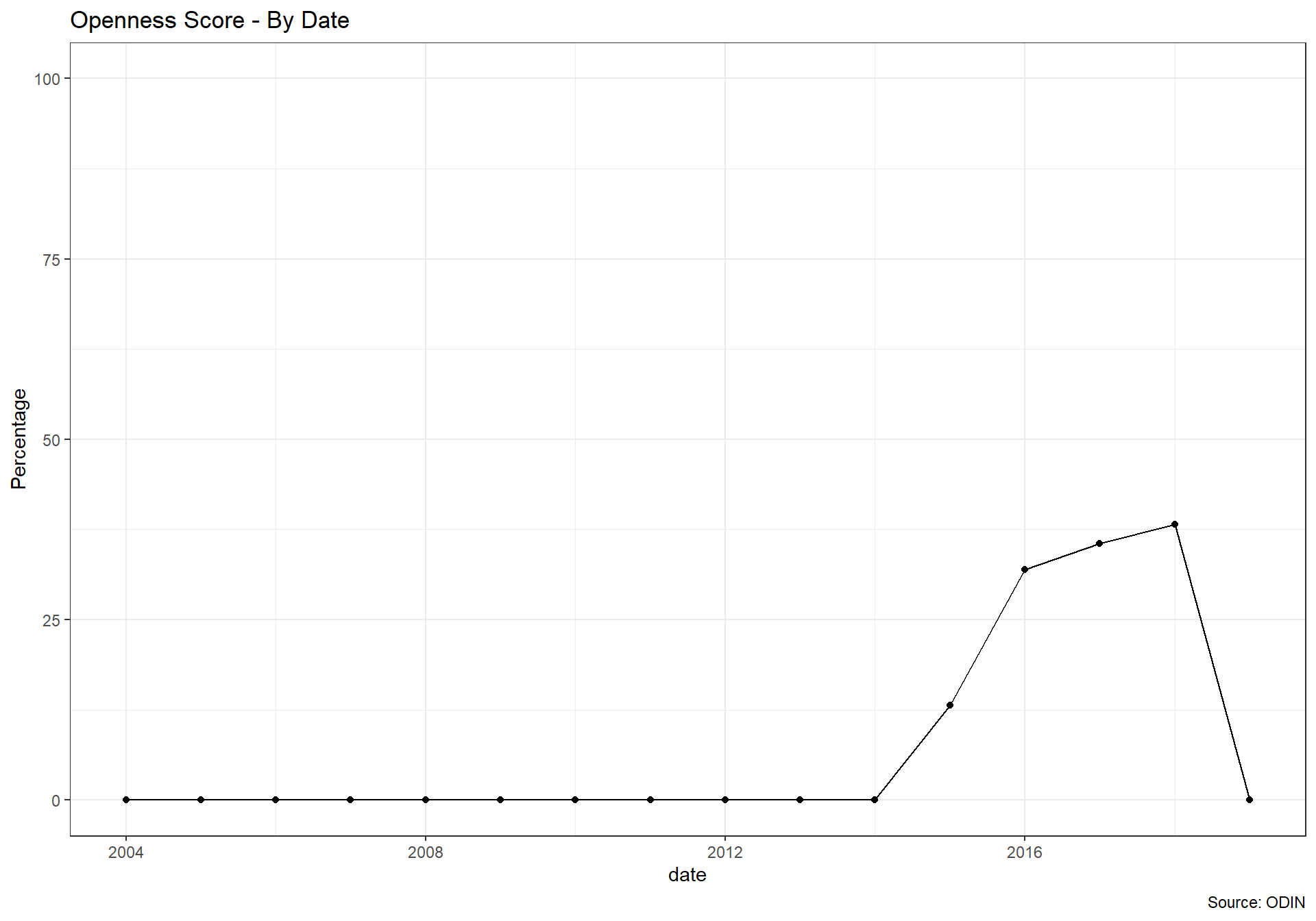
  #read in ODIN data
  for (i in 2015:2018) {
   temp <- read_csv(paste(raw_dir, '/2.2_DSOA/','ODIN_',i,'.csv', sep=""))  %>%
        as_tibble(.name_repair = 'universal') %>%
        mutate(date=i) %>%
        filter(Data.categories=='All Categories')

    assign(paste('openness_df',i,sep="_"), temp)
  }

#bind different years together
openness_df <- bind_rows(openness_df_2015, openness_df_2016, openness_df_2017, openness_df_2018)


openness_df <- openness_df %>%
    select(Country.Code, date, Machine.readable, Non.proprietary, Download.options, Metadata.available, Terms.of.use, Openness.subscore) %>%
    rename(iso3c=Country.Code) %>%
    group_by( iso3c) %>%
    right_join(country_metadata) %>%
    mutate(
      across(c('Machine.readable', 'Non.proprietary', 'Download.options', 'Metadata.available', 'Terms.of.use', 'Openness.subscore'),~if_else(is.na(.), 0, .)           )

           )

#do some quick renaming and formatting
openness_df_temp1 <- openness_df %>%
  rename_with(~paste('RAW.D2.2',., sep="."), .cols=c('Machine.readable', 'Non.proprietary', 'Download.options', 'Metadata.available', 'Terms.of.use', 'Openness.subscore') )


openness_df_temp2 <- openness_df %>%
  mutate(across(c('Machine.readable', 'Non.proprietary', 'Download.options', 'Metadata.available', 'Terms.of.use', 'Openness.subscore'), ~./100)) %>%
  rename_with(~paste('SPI.D2.2',., sep="."), .cols=c('Machine.readable', 'Non.proprietary', 'Download.options', 'Metadata.available', 'Terms.of.use', 'Openness.subscore') )

openness_df <- openness_df_temp1 %>%
  left_join(openness_df_temp2)

#add to spi dataframe
spi_df <- spi_df %>%
  left_join(openness_df)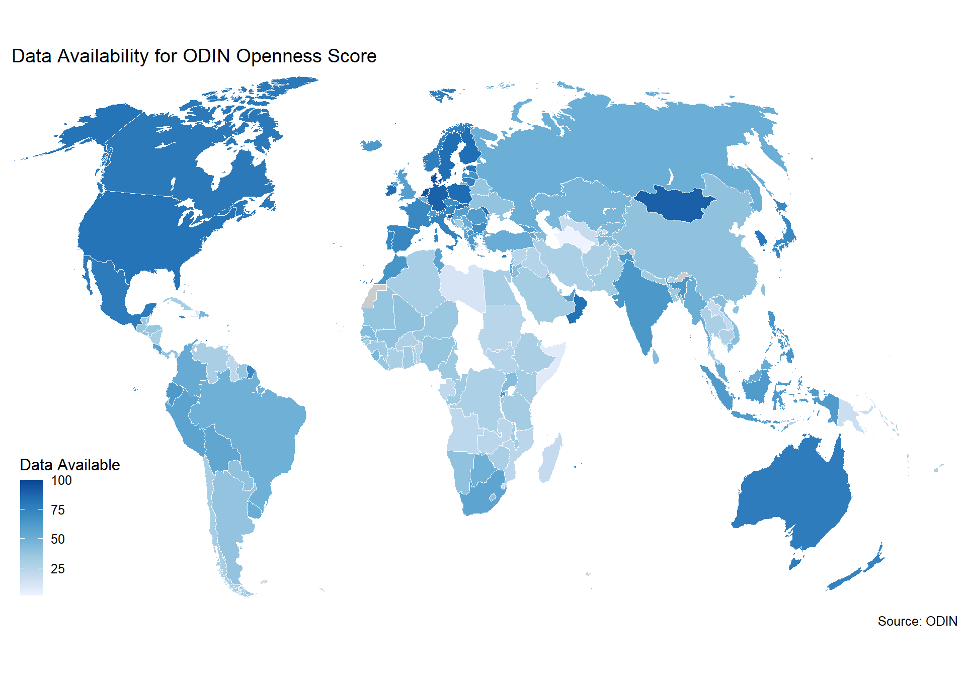
2.2.3 Indicator 2.3: Advisory/ Analytical Services
No established source exists for this indicator. This is experimental.
2.2.4 Indicator 2.4: Data services
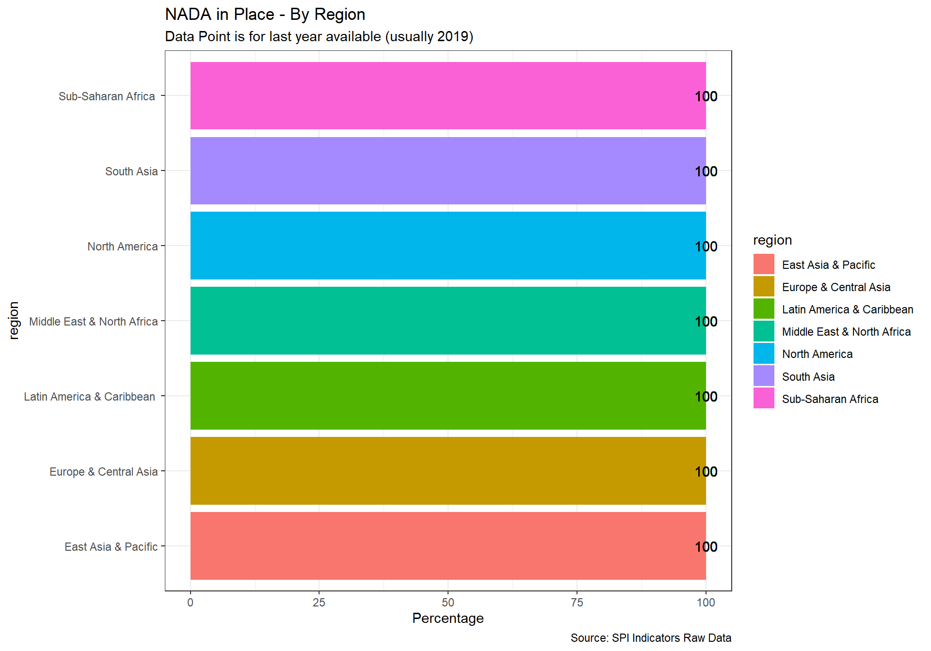
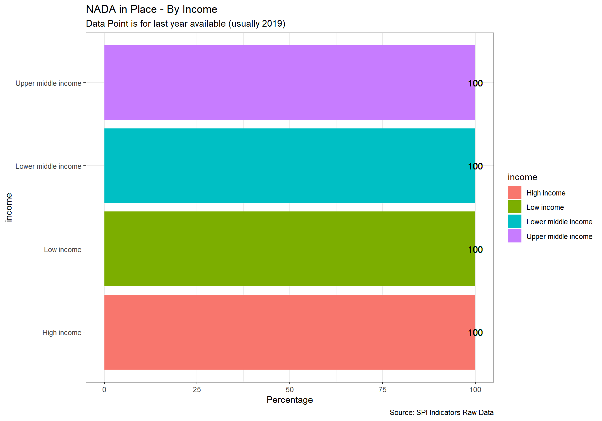
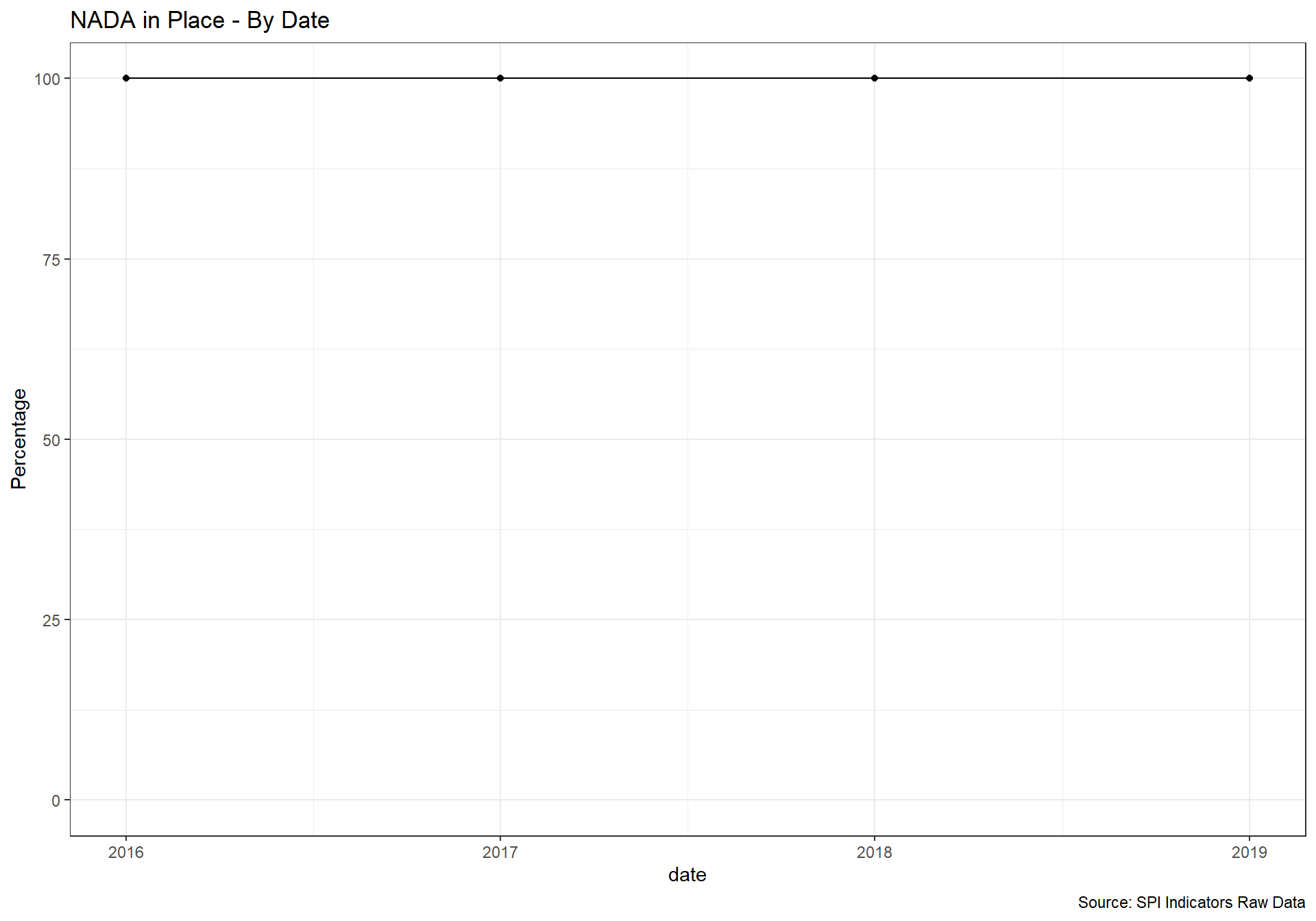
NSO has a listing of surveys and microdata sets that can provide the necessary data and reference for follow-up. Upon well-defined request and procedure per the national law and practice, users and practitioners can obtain the data collected from the households and businesses when needed.
NADA is an open source microdata cataloging system, compliant with the Data Documentation Initiative (DDI) and Dublin Core’s RDF metadata standards. It serves as a portal for researchers to browse, search, compare, apply for access, and download relevant census or survey datasets, questionnaires, reports and other information.
1 Point. Yes 0 Points. No
#read in csv file.
D2.4_NADA <- read_csv(file = paste(raw_dir, '/2.4_DSDS/', "D2.4.NADA.csv", sep="/" )) %>%
  mutate(SPI.D2.4.NADA=case_when(
    NADA==1 ~ 1,
    NADA==0 ~ 0,
    TRUE ~ 0
  ))  %>%
  rename(RAW.D2.4.NADA=NADA,
         RAW.D2.4.NADA_text=NADA_text) %>%
  select(iso3c, country, date, RAW.D2.4.NADA,RAW.D2.4.NADA_text, SPI.D2.4.NADA  ) %>%
  arrange(date, country)

D2.4_NADA_map <- D2.4_NADA %>%
  filter(SPI.D2.4.NADA>0)

spi_mapper('D2.4_NADA_map', 'RAW.D2.4.NADA', 'NADA in Place' )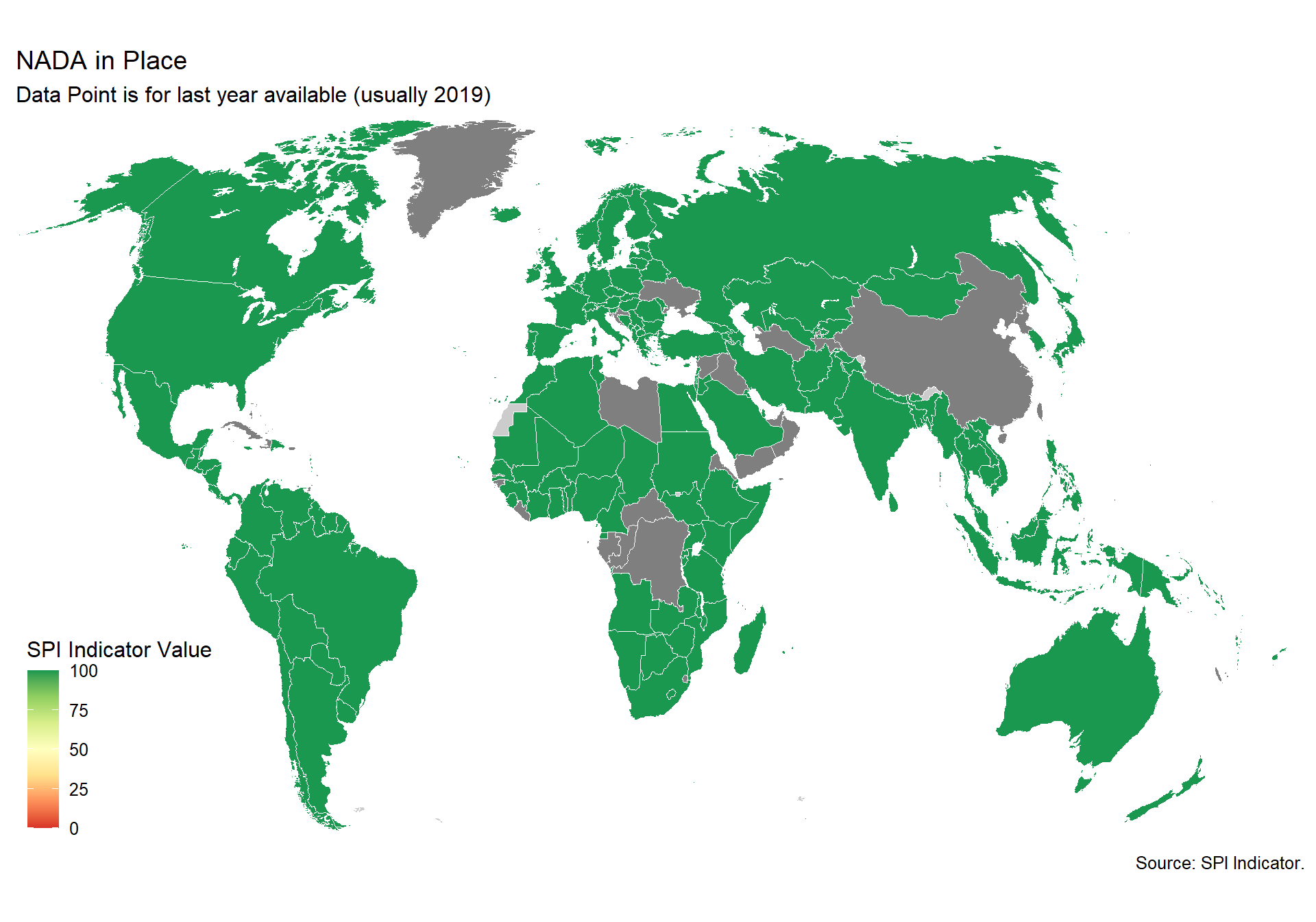
#add to spi databases
spi_df <- spi_df %>%
  left_join(D2.4_NADA)
2.3 Data Products
Cleaning for Data Products Indicators. Data Products (16 Indicators):
- GOAL 1: No Poverty
- GOAL 2: Zero Hunger
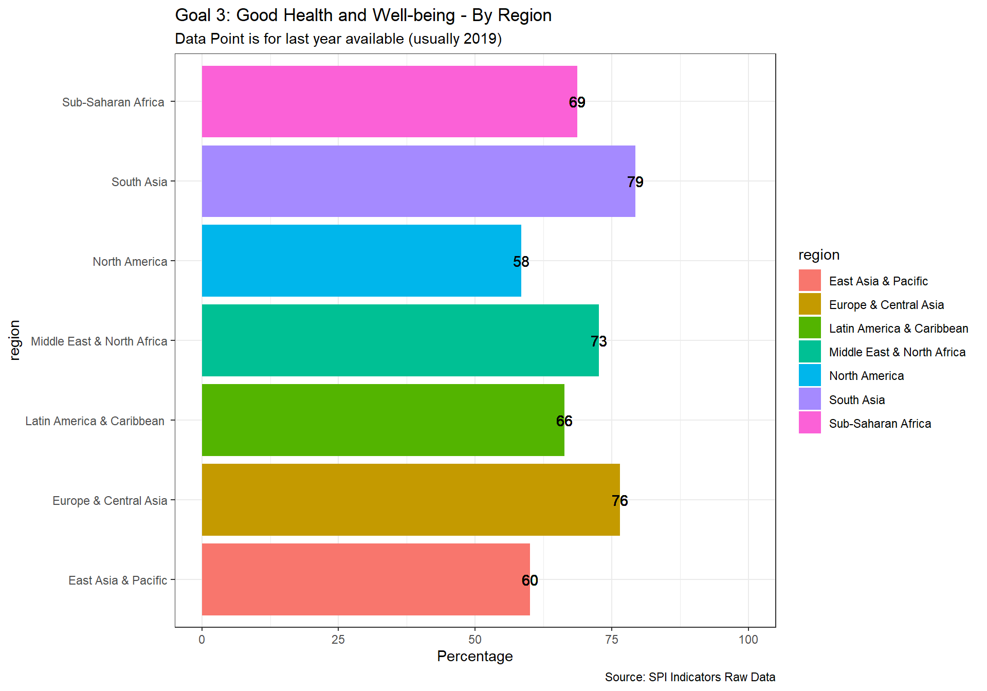
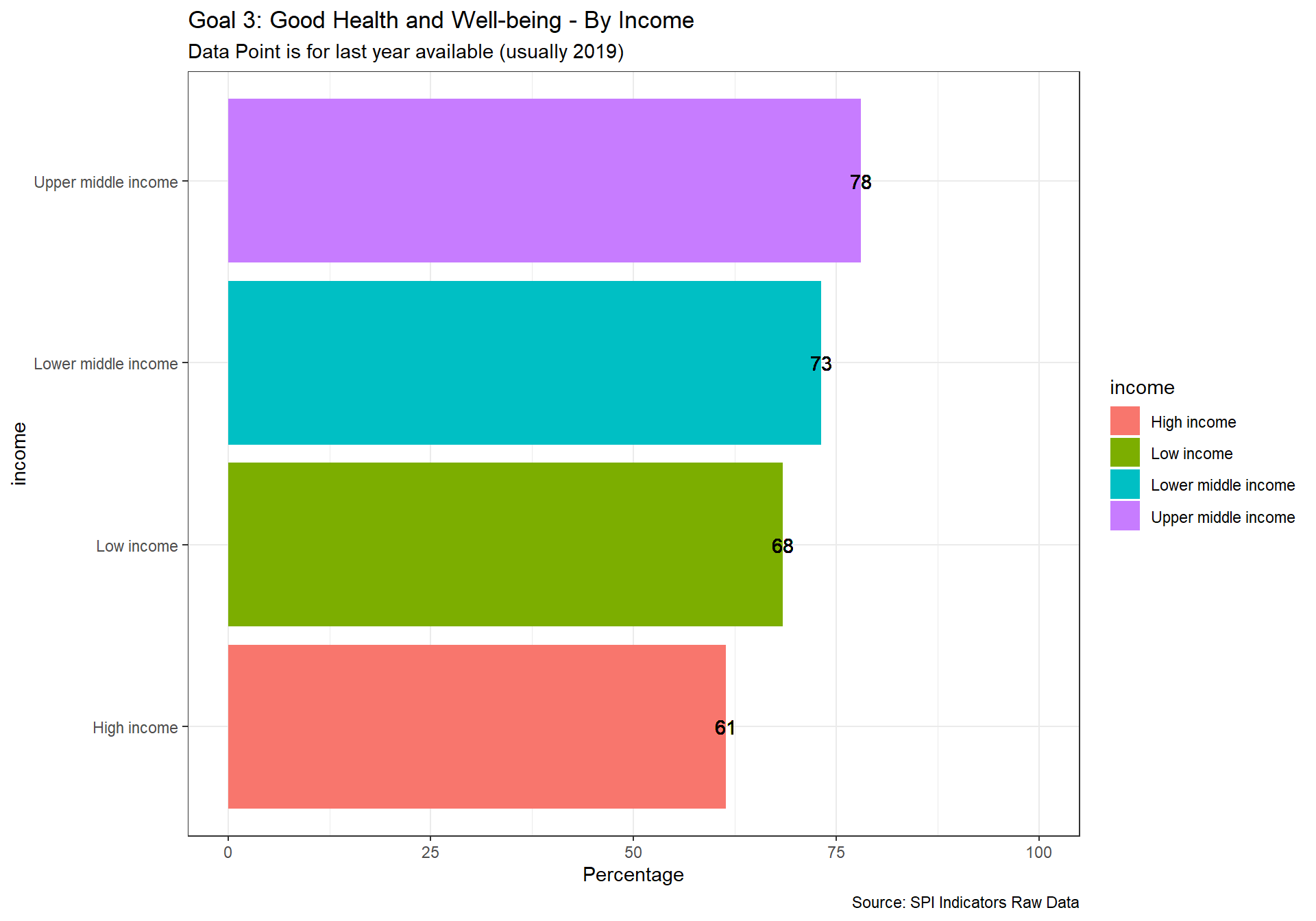
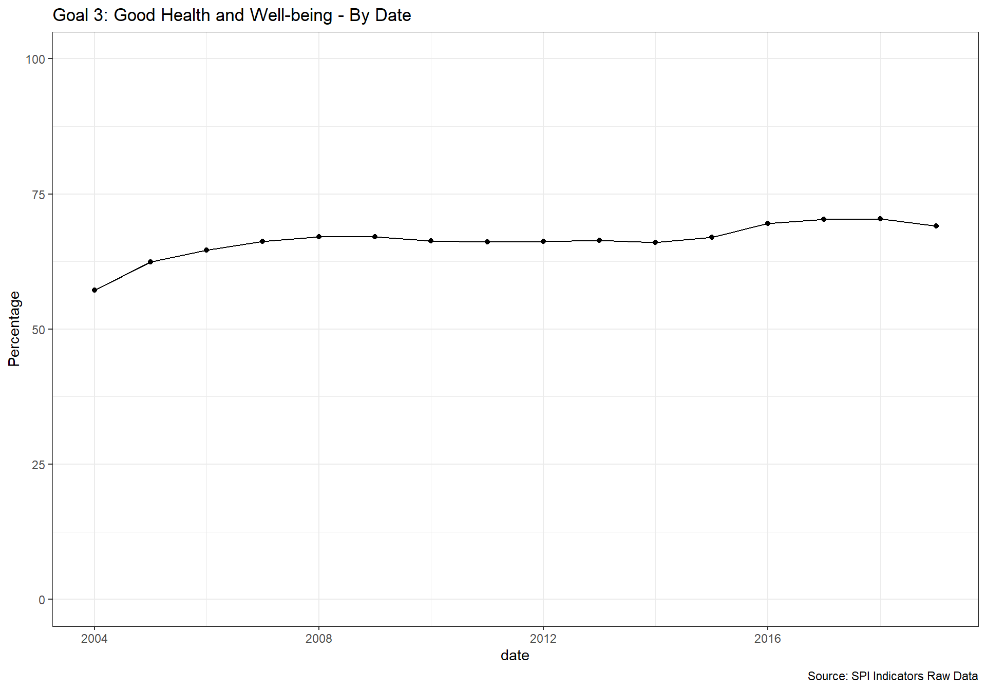
- GOAL 3: Good Health and Well-beingq
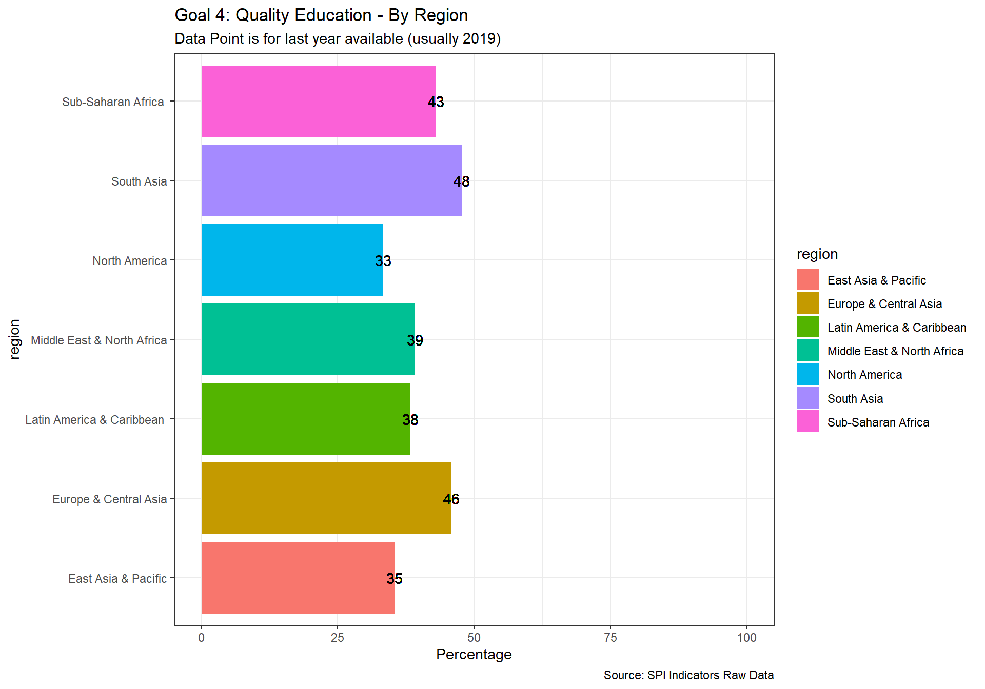
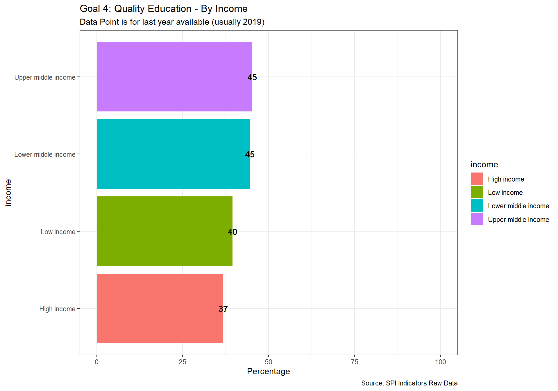
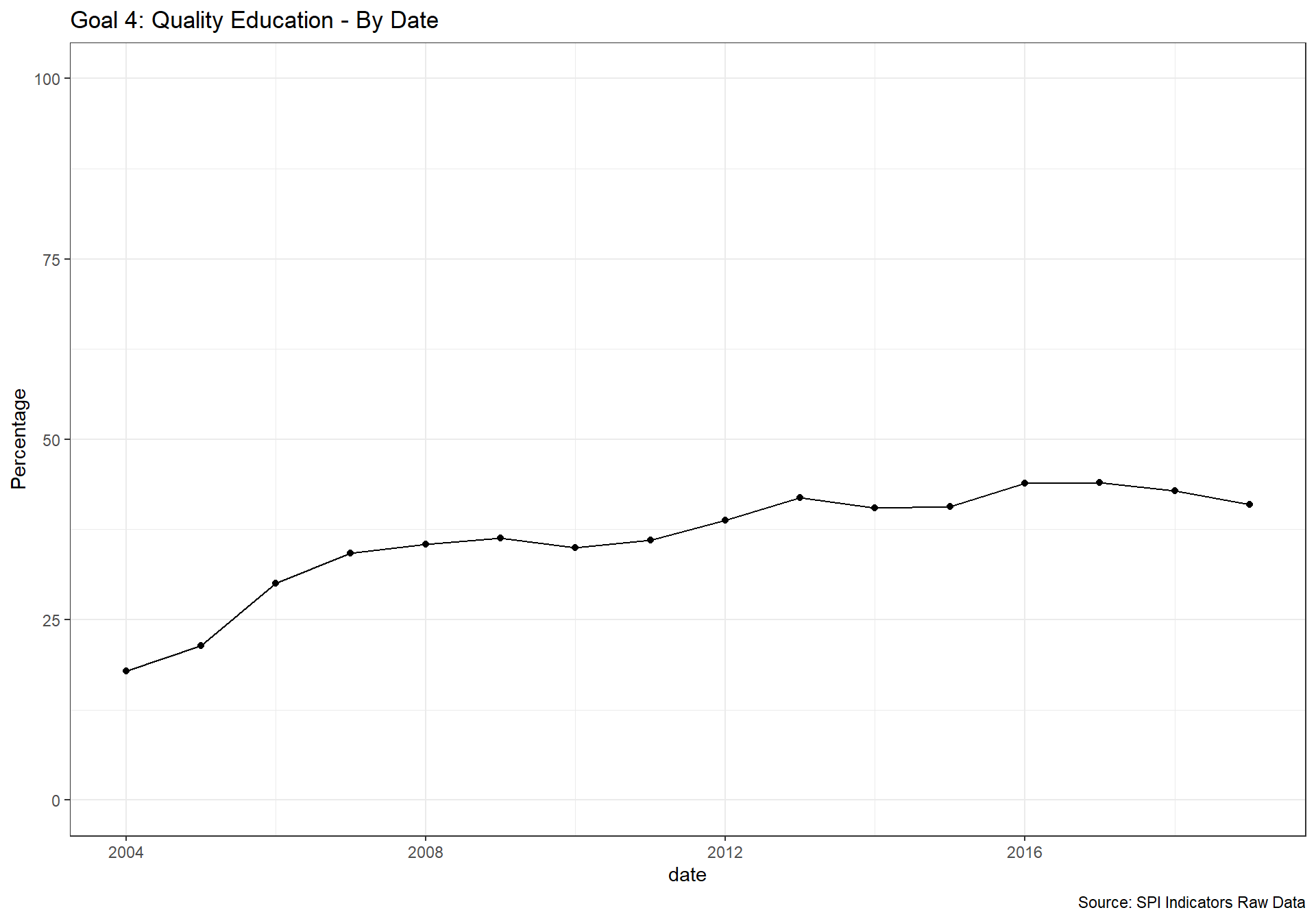
- GOAL 4: Quality Education
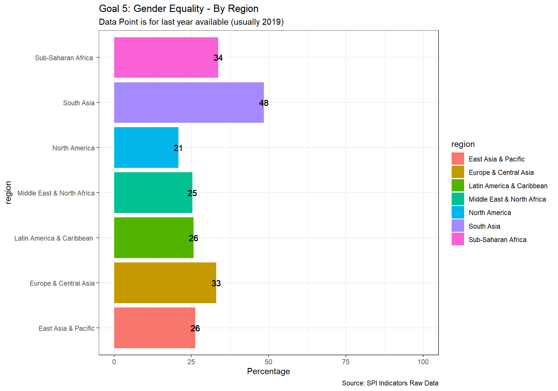
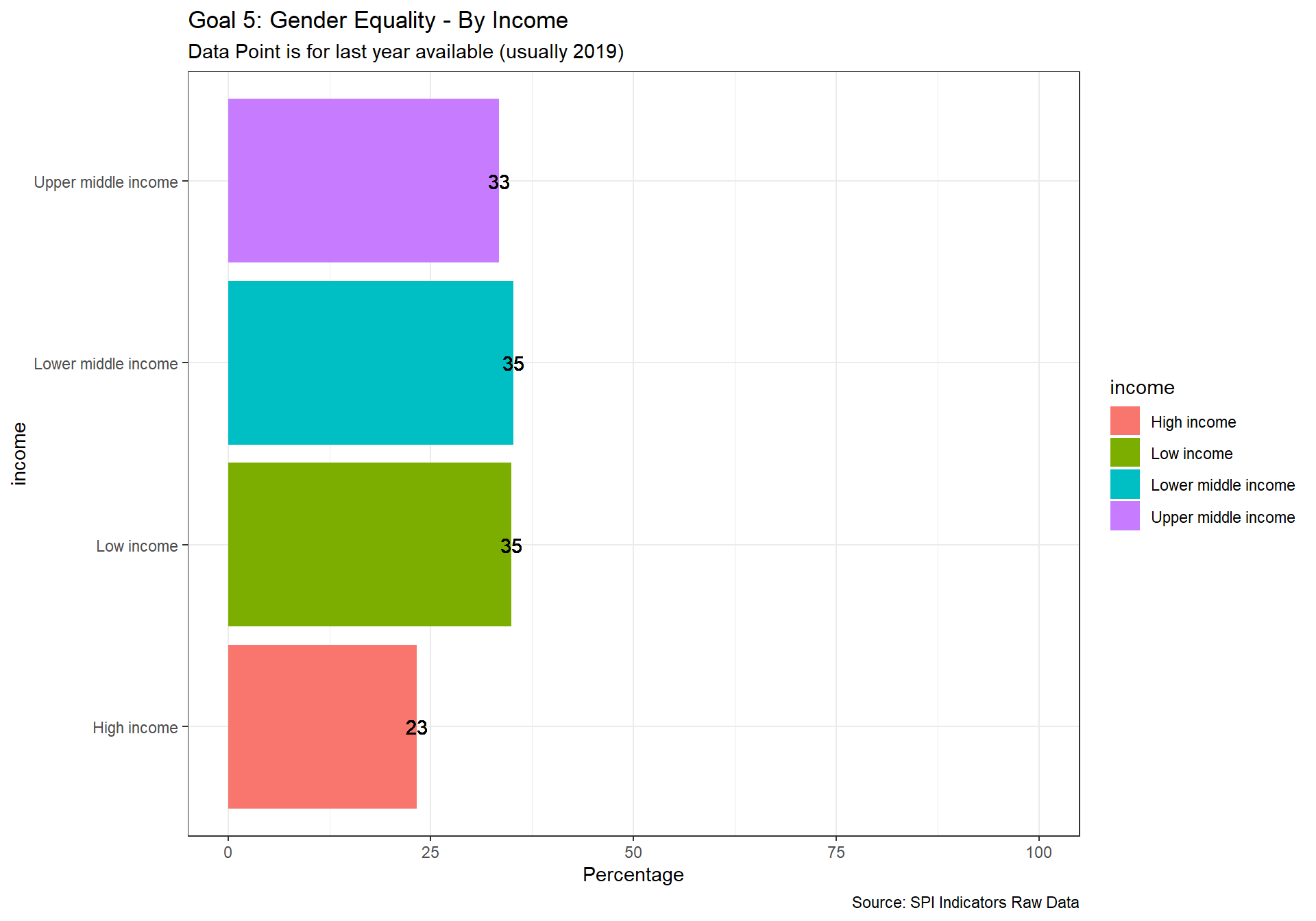
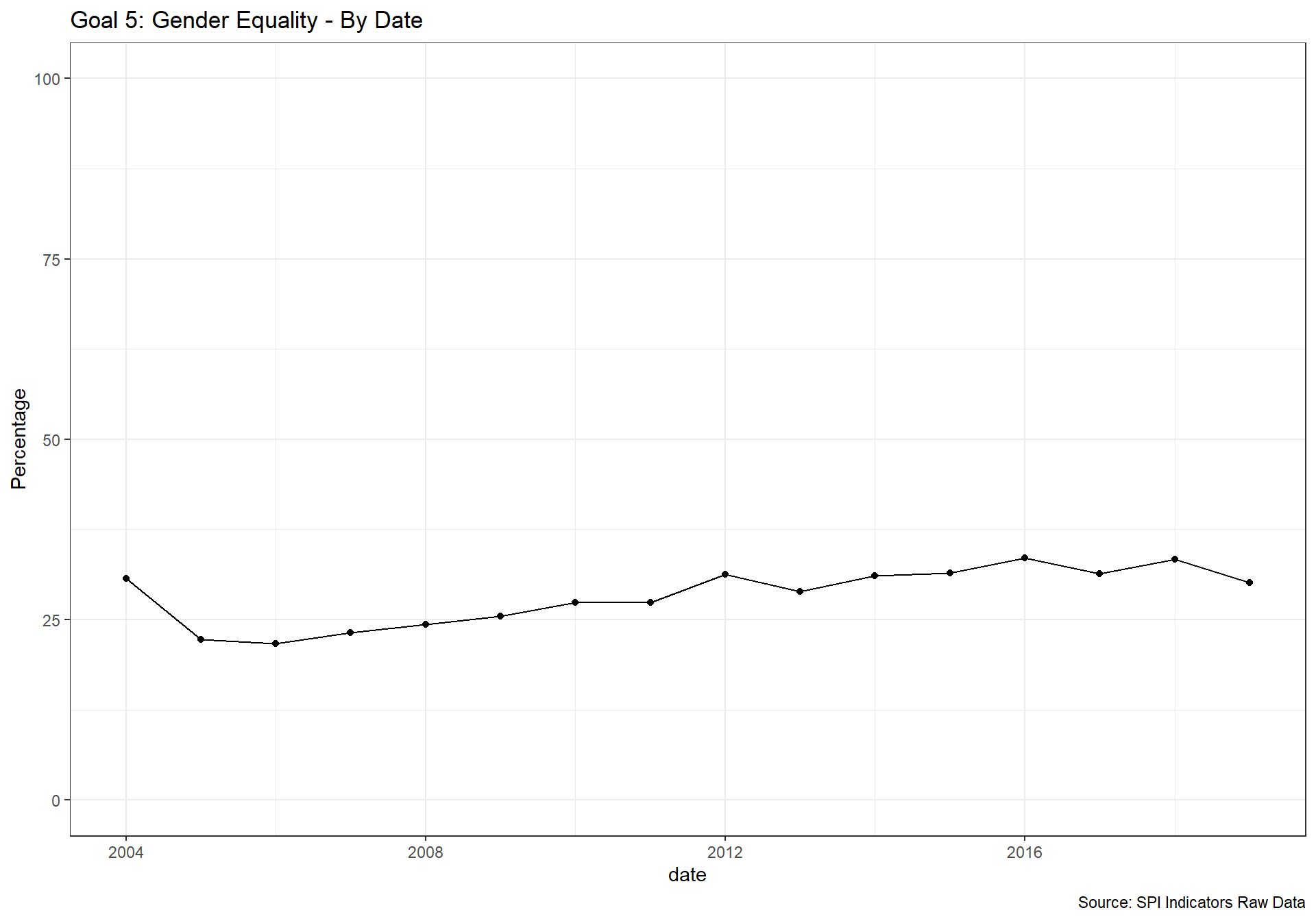
- GOAL 5: Gender Equality
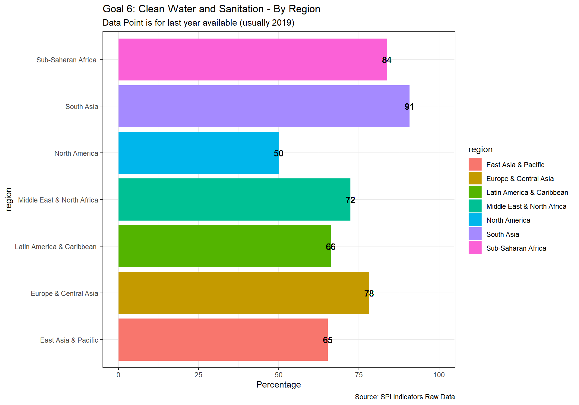
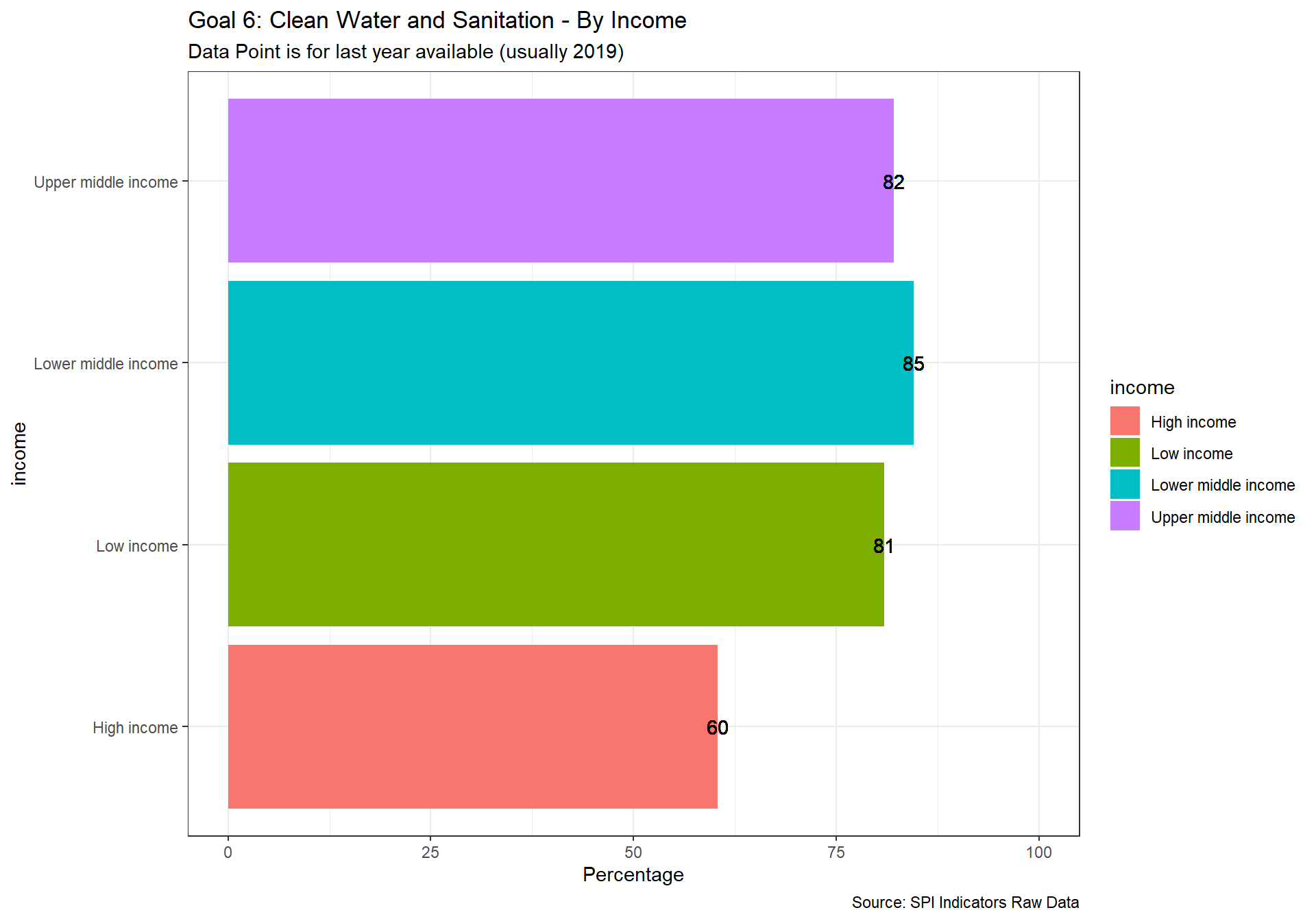
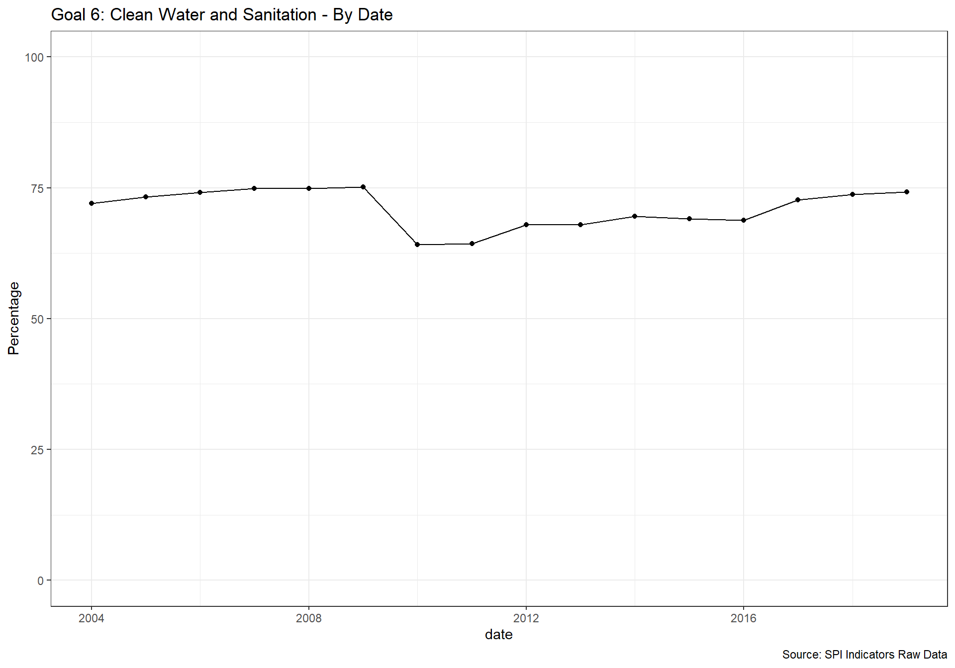
- GOAL 6: Clean Water and Sanitation
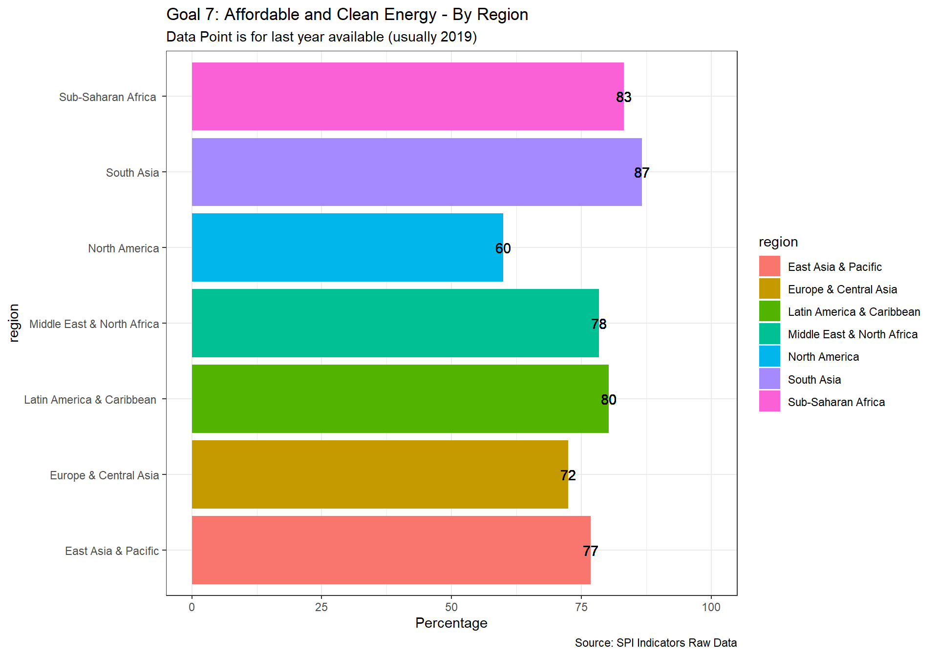
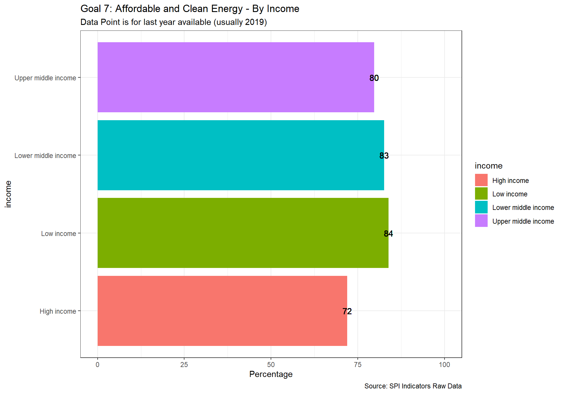
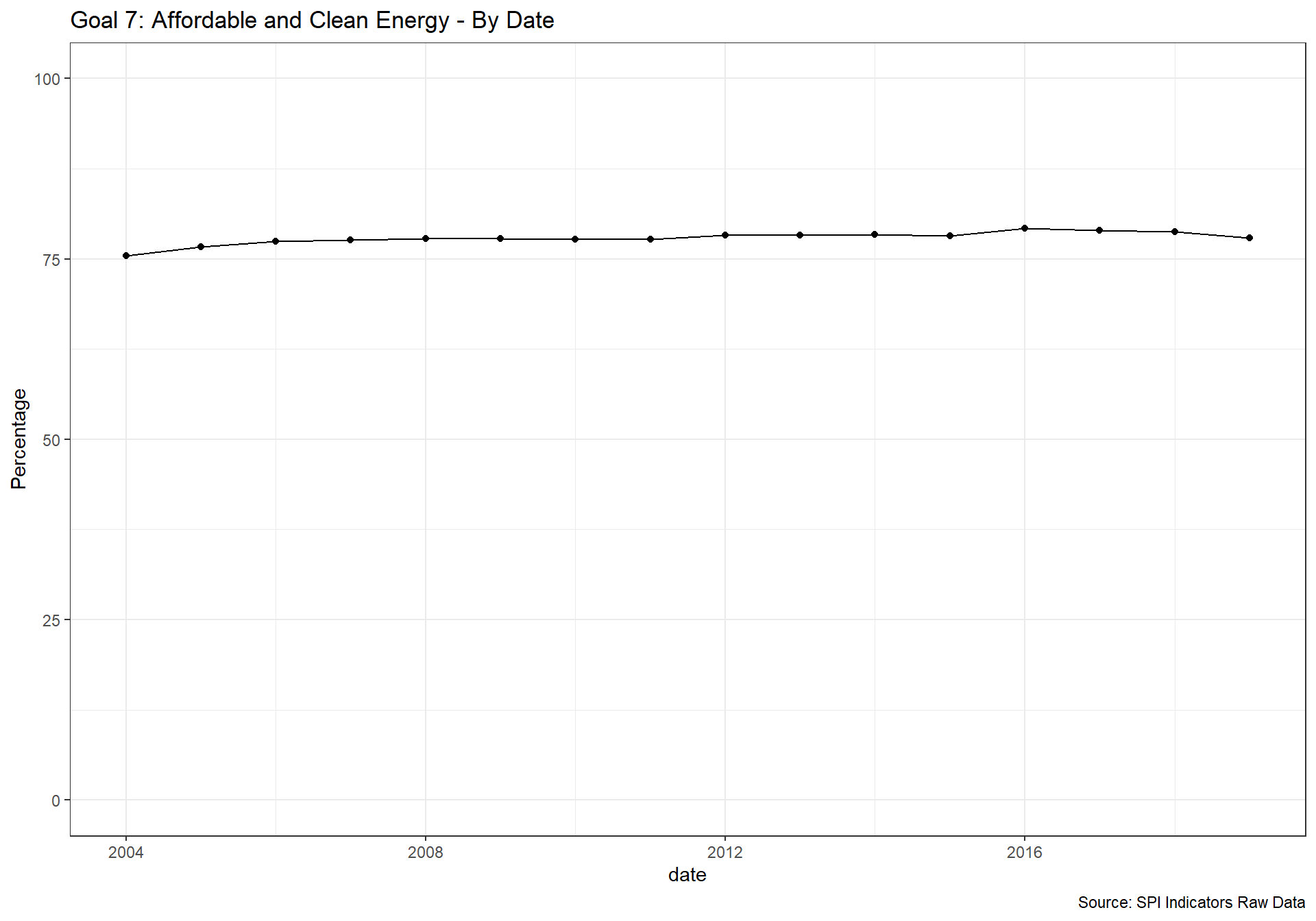
- GOAL 7: Affordable and Clean Energy
- GOAL 8: Decent Work and Economic Growth
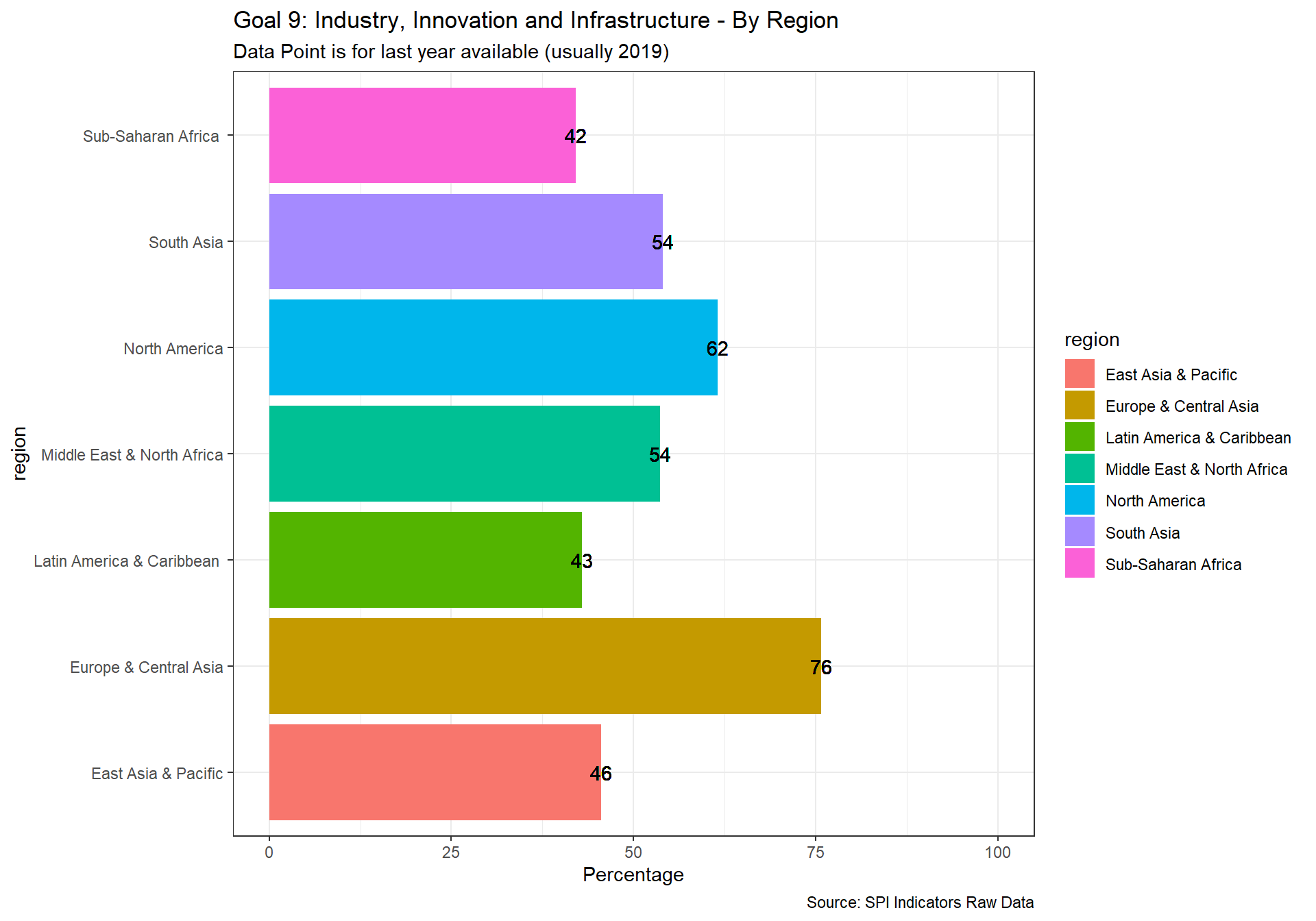
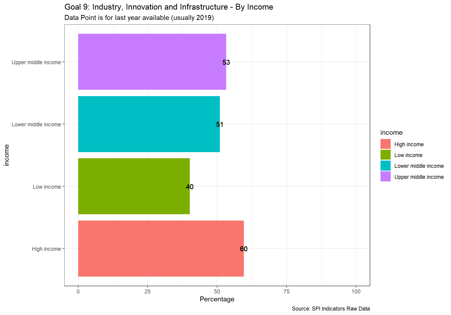
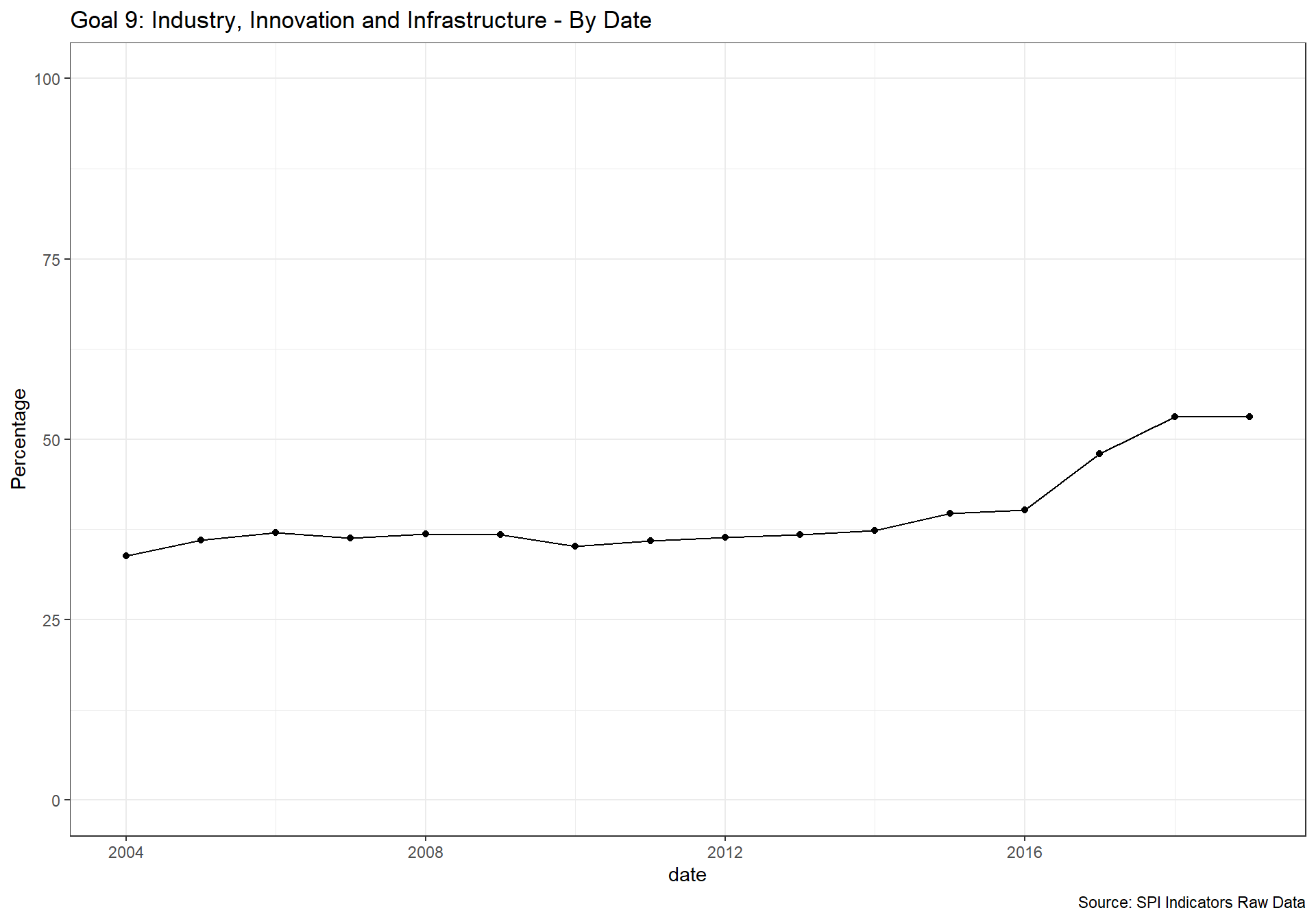
- GOAL 9: Industry, Innovation and Infrastructure
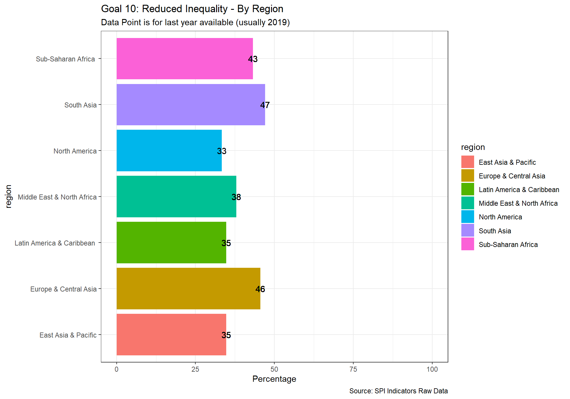
- GOAL 10: Reduced Inequality
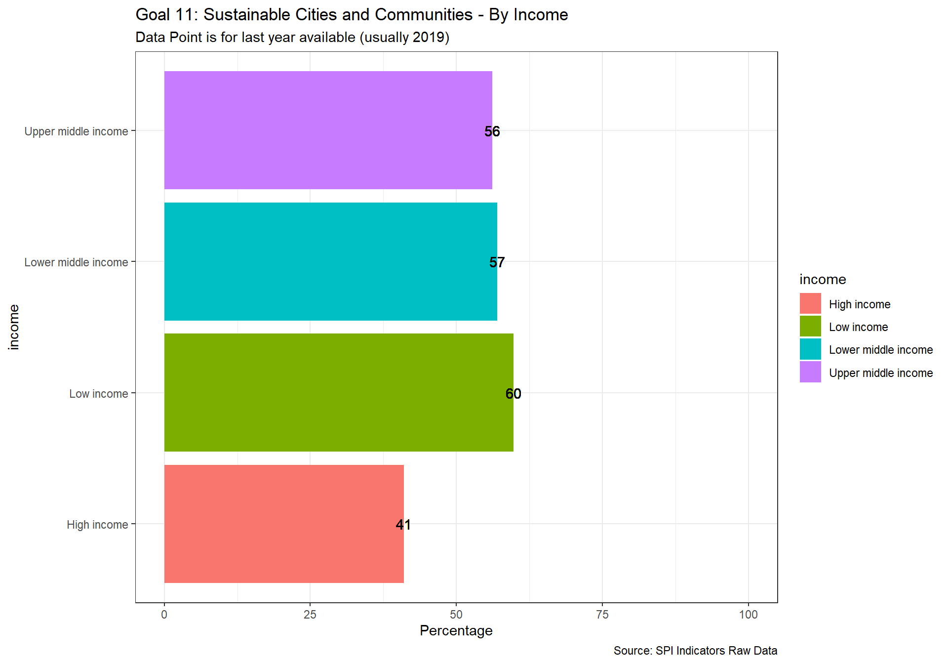
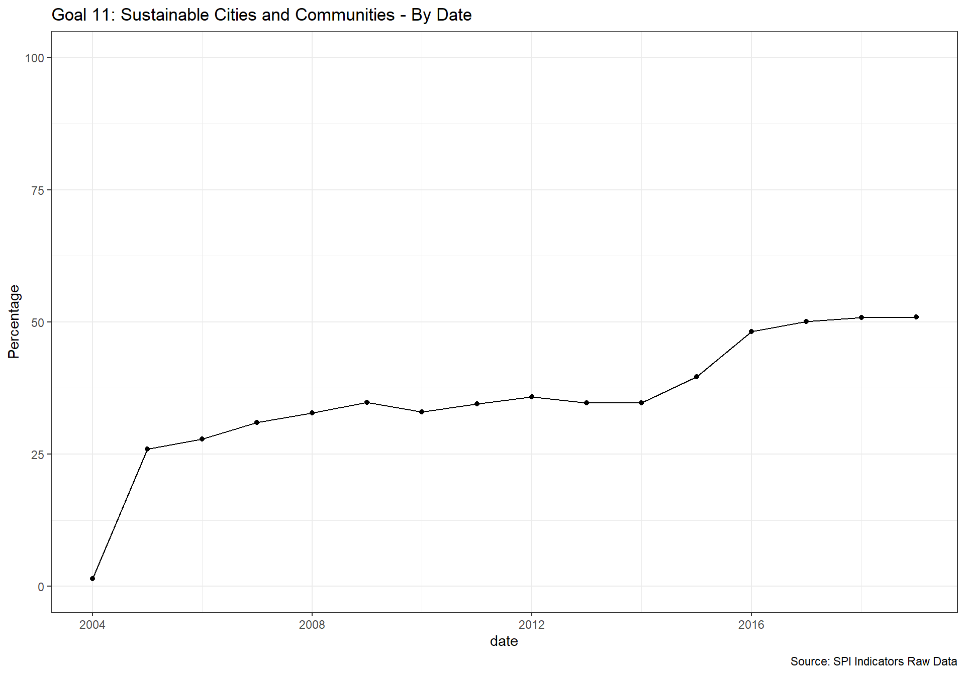
- GOAL 11: Sustainable Cities and Communities
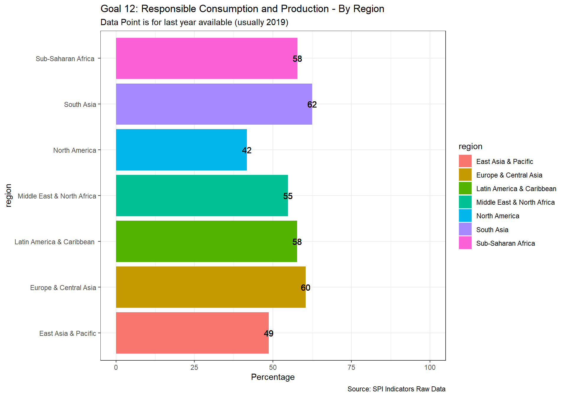
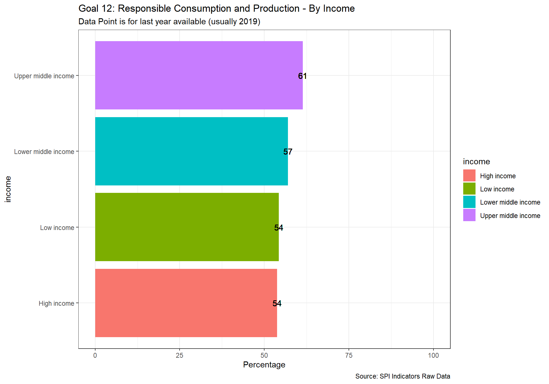
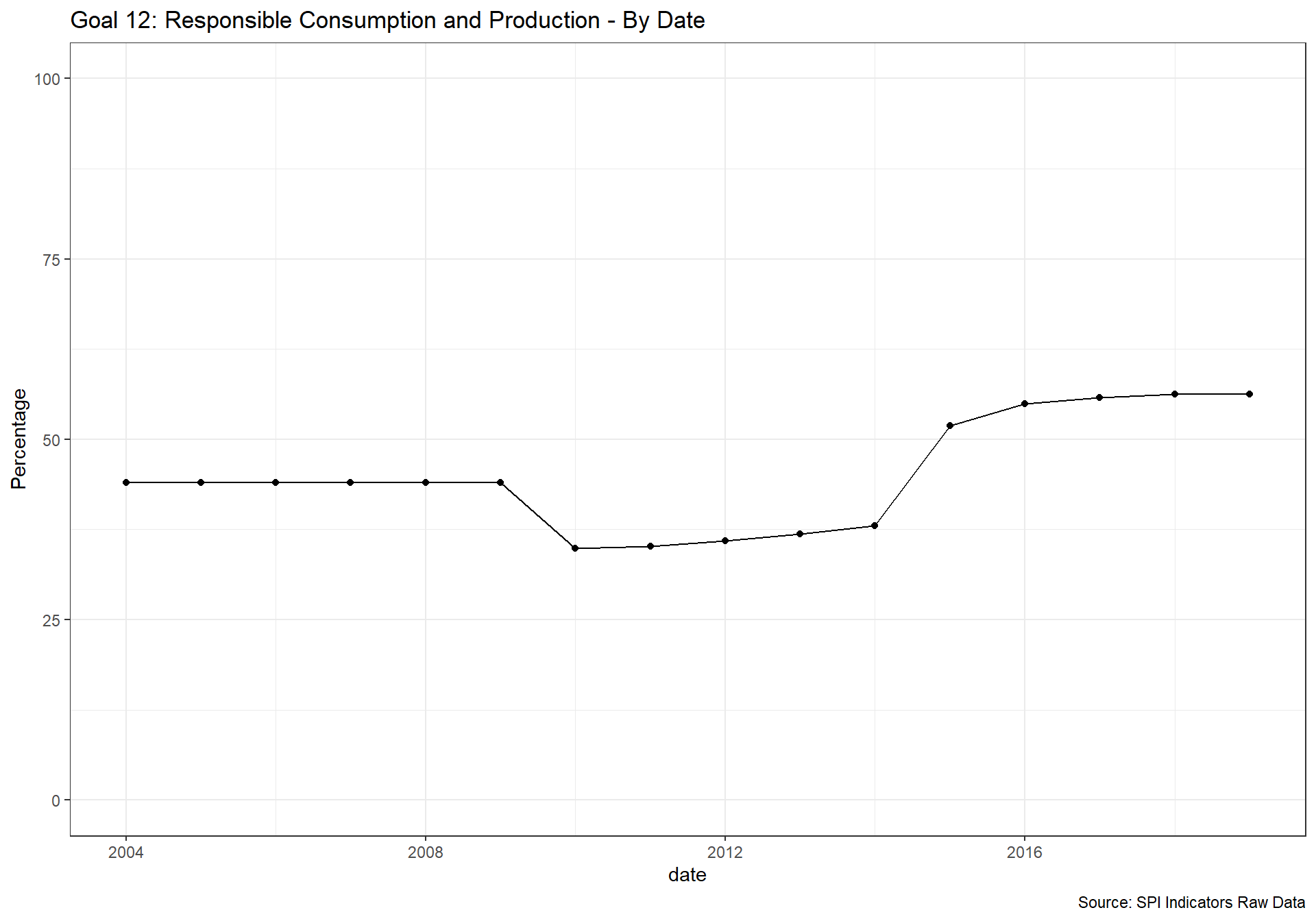
- GOAL 12: Responsible Consumption and Production
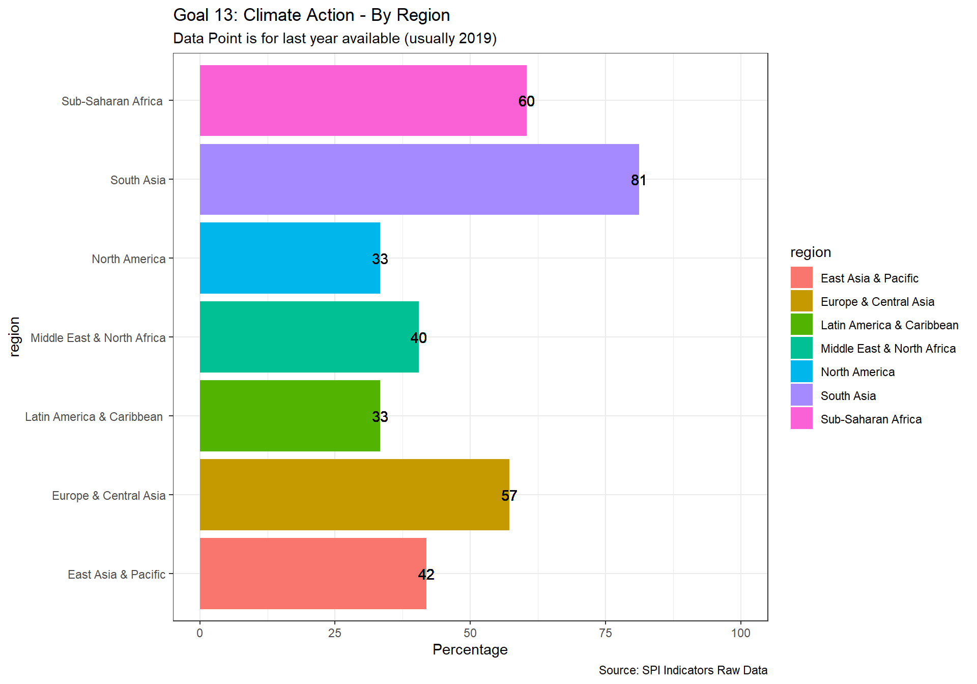
- GOAL 13: Climate Action
- GOAL 14: Life Below Water is excluded because this indicator is not relevant for landlocked countries
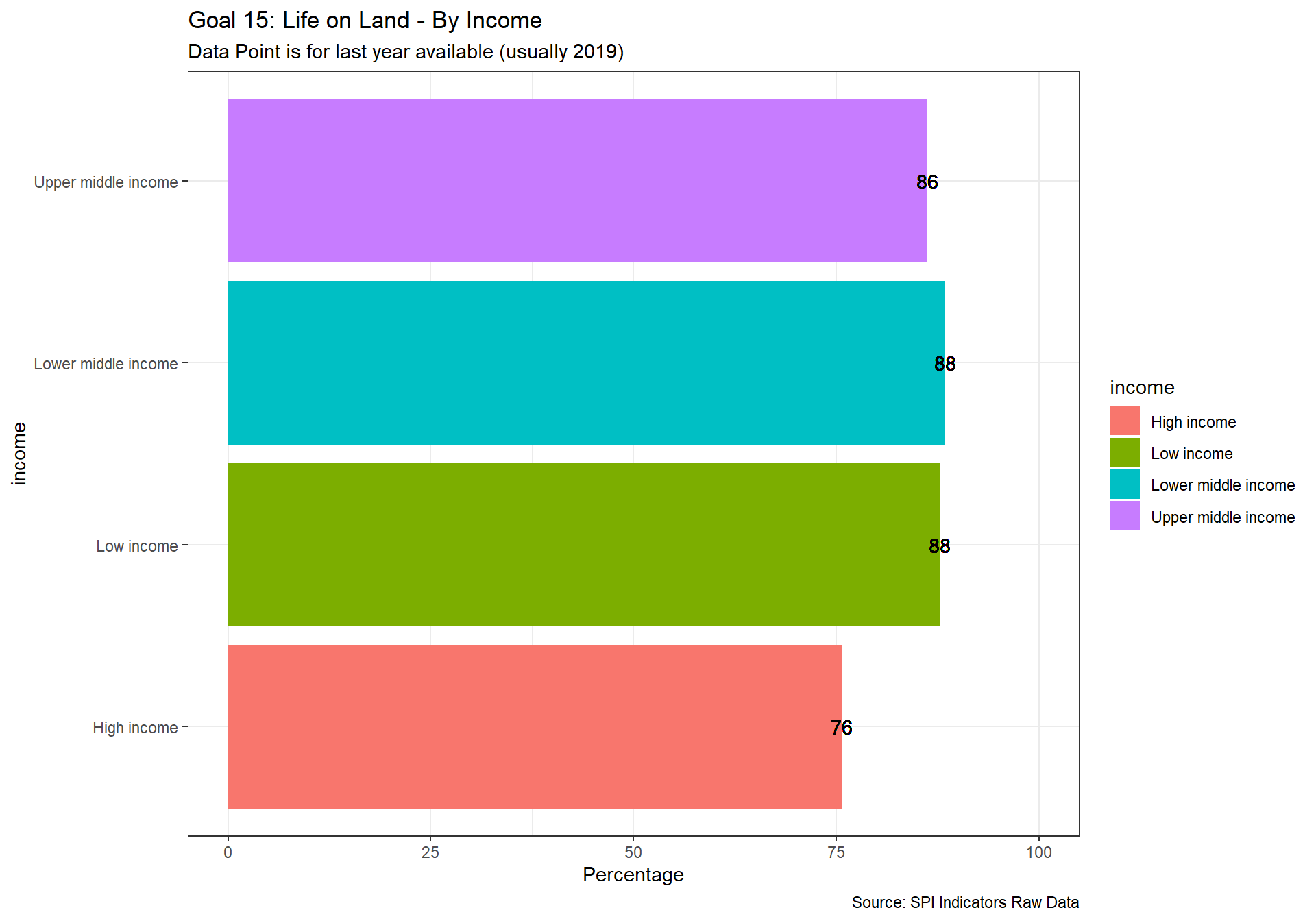
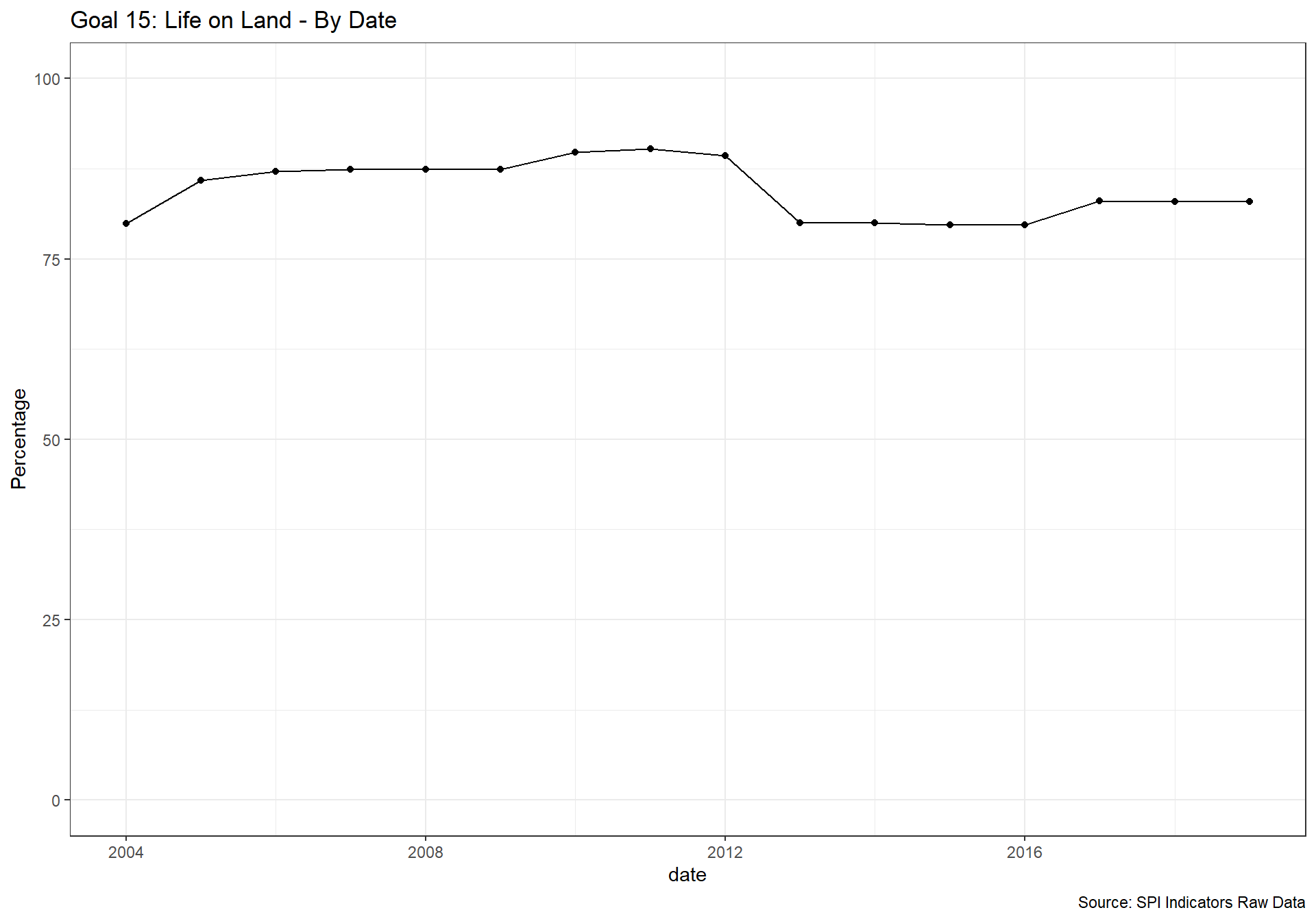
- GOAL 15: Life on Land
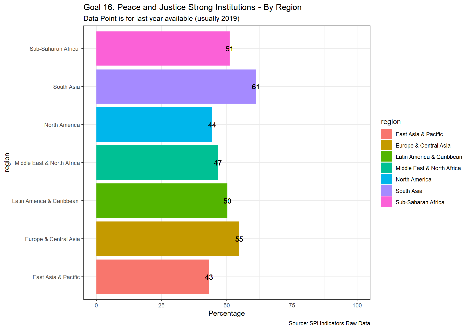
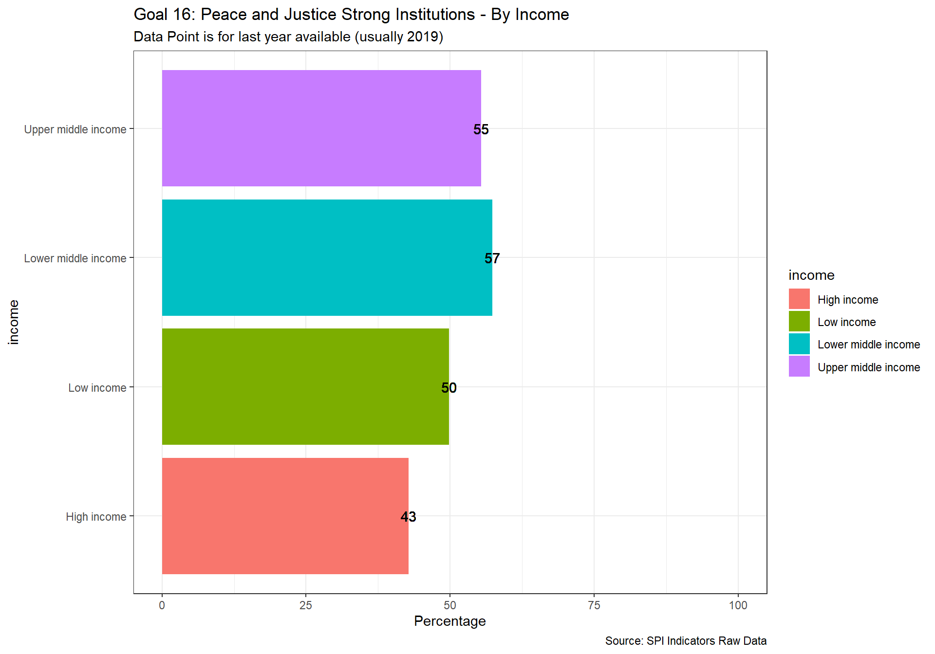
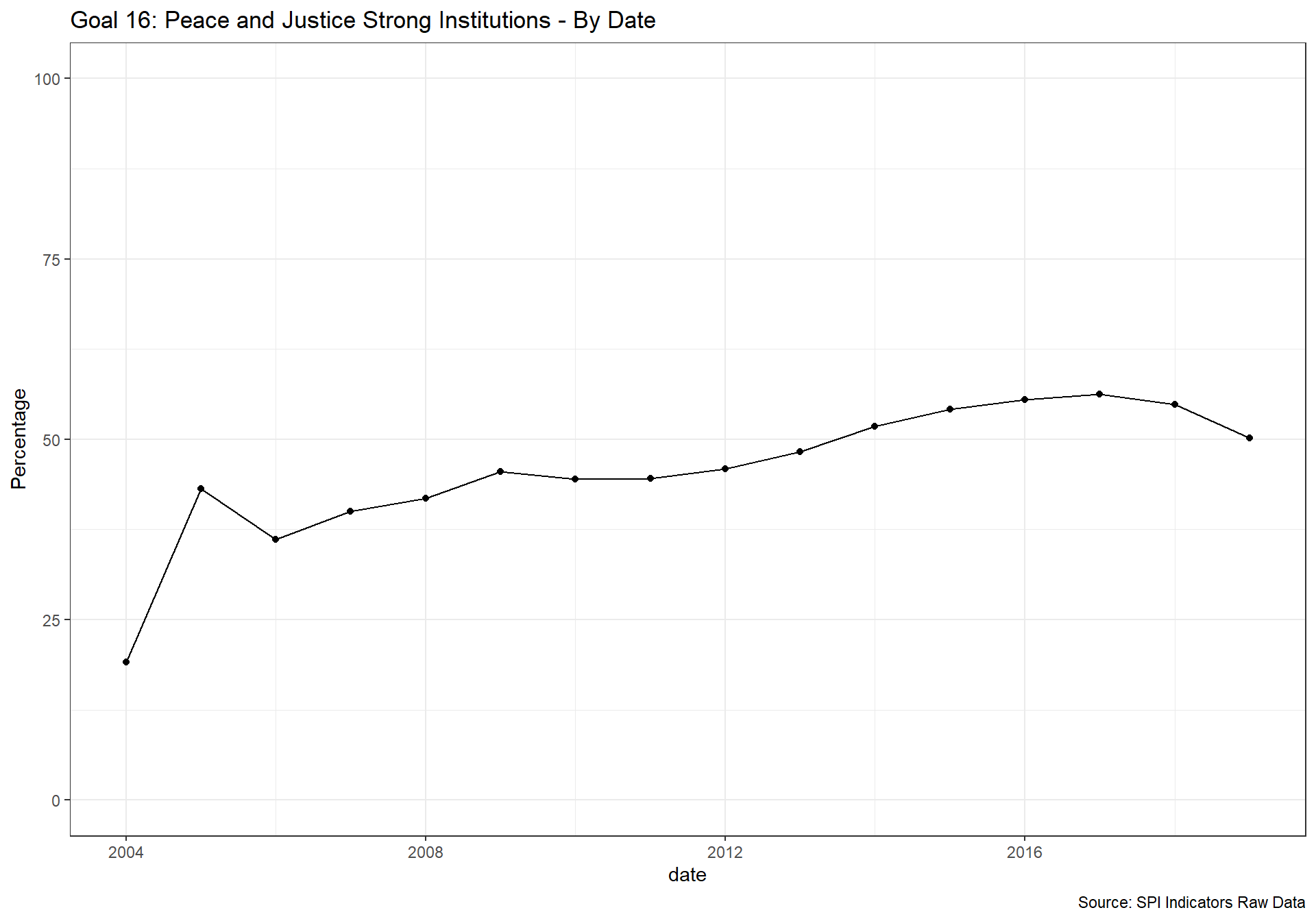
- GOAL 16: Peace and Justice Strong Institutions
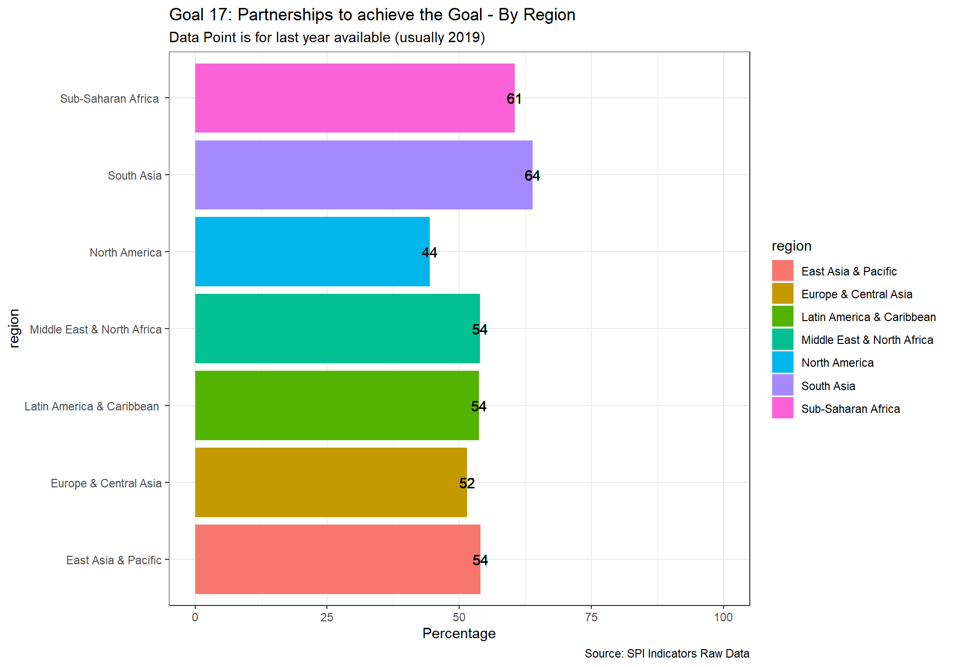
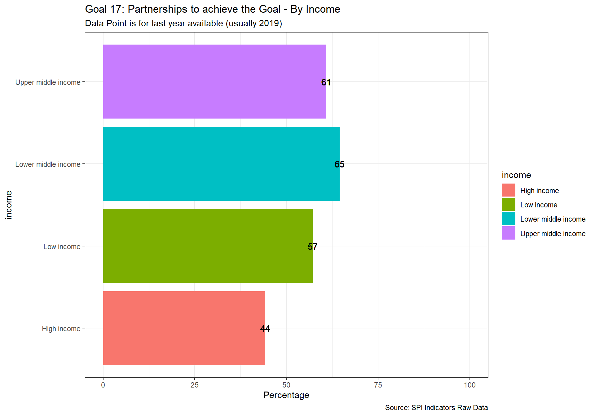
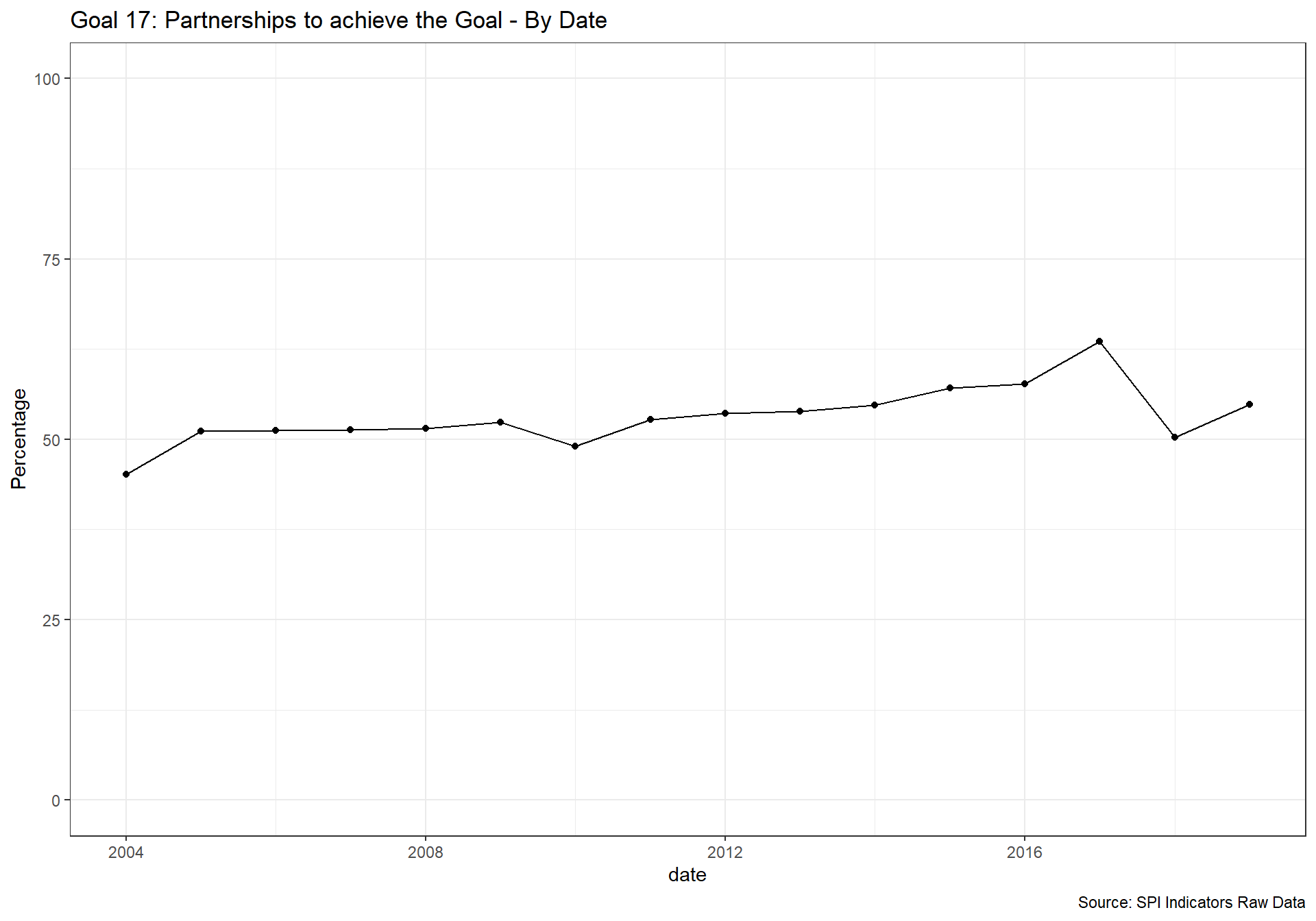
- GOAL 17: Partnerships to achieve the Goal
2.3.1 Methodology
Download the latest SDG indicator data from UN Stats (https://unstats.un.org/sdgs/indicators/en/#) using their API
Transform the data so that for each indicator we can create a score documenting whether a value exists for the country in a year, whether the value is based on country data, country data adjusted, estimated, or modelled data according the UN Stats metadata. This will only include tier 1 indicators.
Combine the resulting data into a single set of indicators for use in the Statistical Performance Indicators dashboard and index by calculating the average across SDGs. This results in 17 total indicators. One for each SDG, which is the share of indicators with a value meeting quality criteria defined below.
Below is a paraphrased description from the UN stats webpage (https://unstats.un.org/sdgs/indicators/indicators-list/):
The global indicator framework for Sustainable Development Goals was developed by the Inter-Agency and Expert Group on SDG Indicators (IAEG-SDGs) and agreed upon at the 48th session of the United Nations Statistical Commission held in March 2017.
The global indicator framework includes 231 unique indicators. Please note that the total number of indicators listed in the global indicator framework of SDG indicators is 247. However, twelve indicators repeat under two or three different targets.
For each value of the indicator, the responsible international agency has been requested to indicate whether the national data were adjusted, estimated, modelled or are the result of global monitoring. The “nature” of the data in the SDG database is determined as follows:
Country data (C): Produced and disseminated by the country (including data adjusted by the country to meet international standards);
Country data adjusted (CA): Produced and provided by the country, but adjusted by the international agency for international comparability to comply with internationally agreed standards, definitions and classifications;
Estimated (E): Estimated based on national data, such as surveys or administrative records, or other sources but on the same variable being estimated, produced by the international agency when country data for some year(s) is not available, when multiple sources exist, or when there are data quality issues;
Modelled (M): Modelled by the agency on the basis of other covariates when there is a complete lack of data on the variable being estimated;
Global monitoring data (G): Produced on a regular basis by the designated agency for global monitoring, based on country data. There is no corresponding figure at the country level.
For each indicator, we will produce a value for each country with the following coding scheme:
- 1 Point: Indicator exists and the value is based on the country, country data adjusted, or estimated or Global Monitoring data
- 0 Points: Indicator based on modeled data or does not exists
We give countries no credit for modeled data, because the country did not produce indicators in a form that was directly usable for reporting on an SDG indicator.
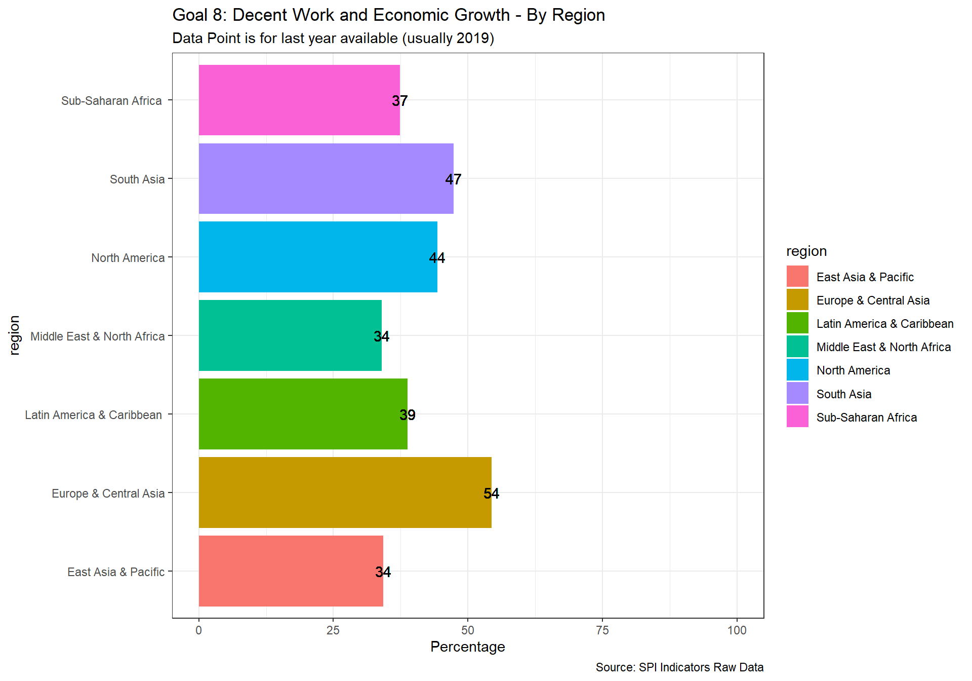
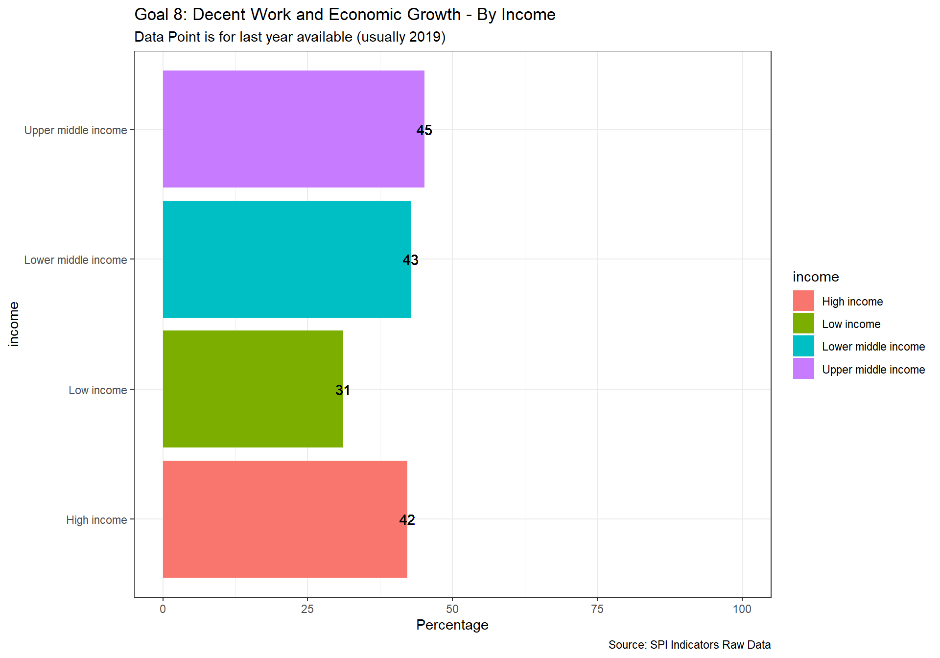
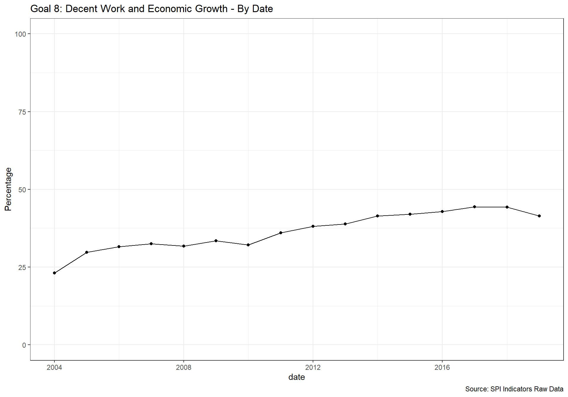
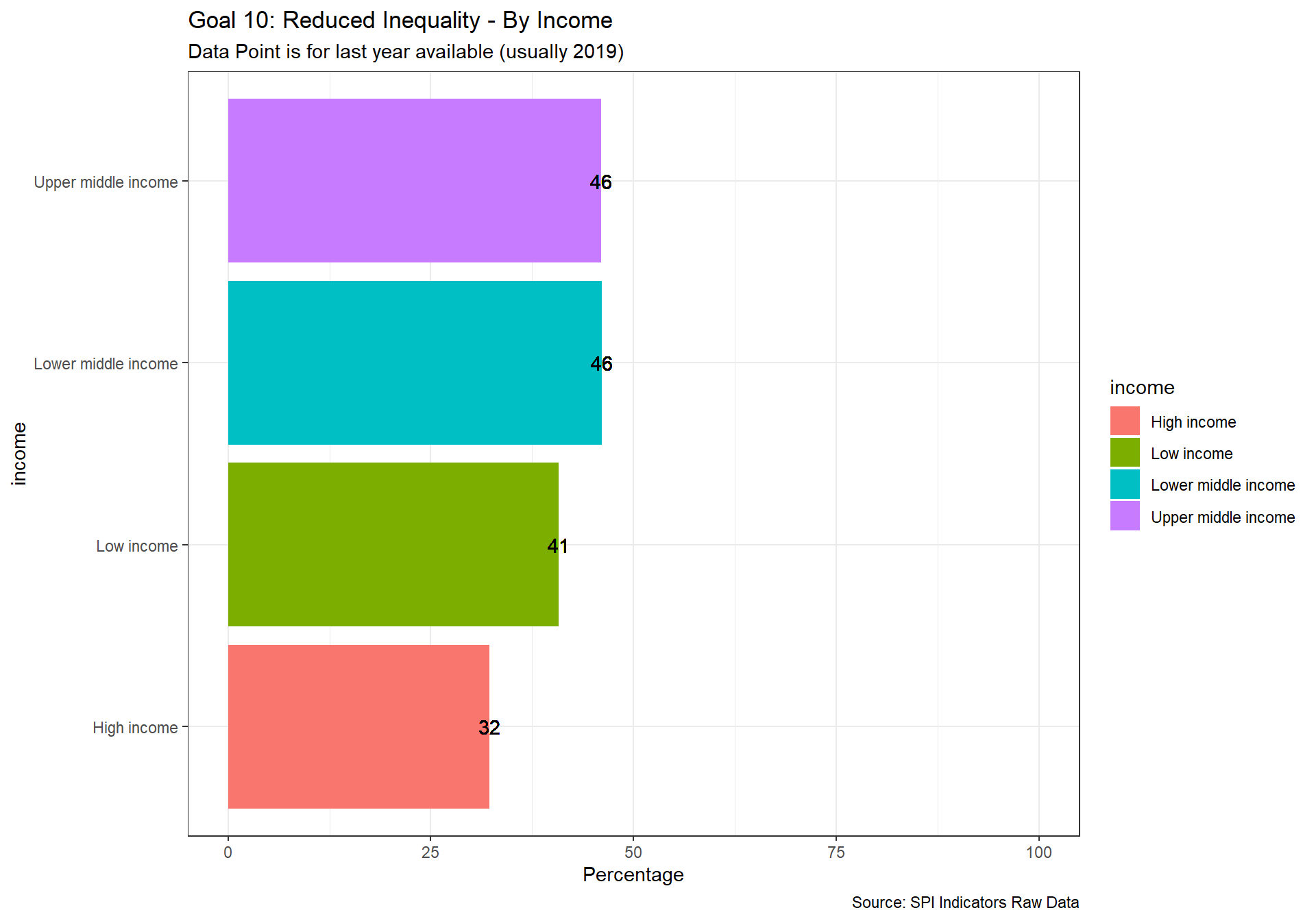
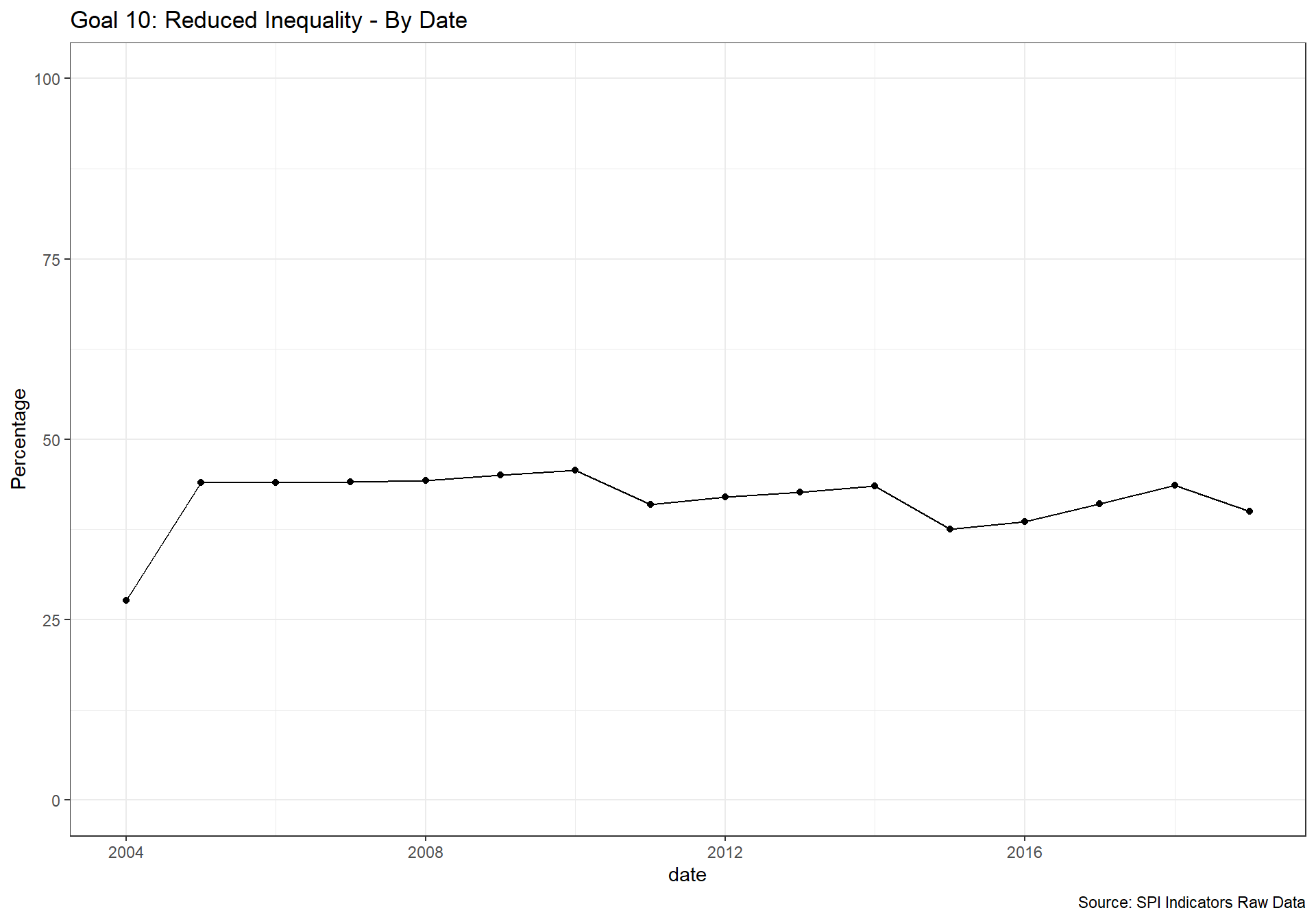
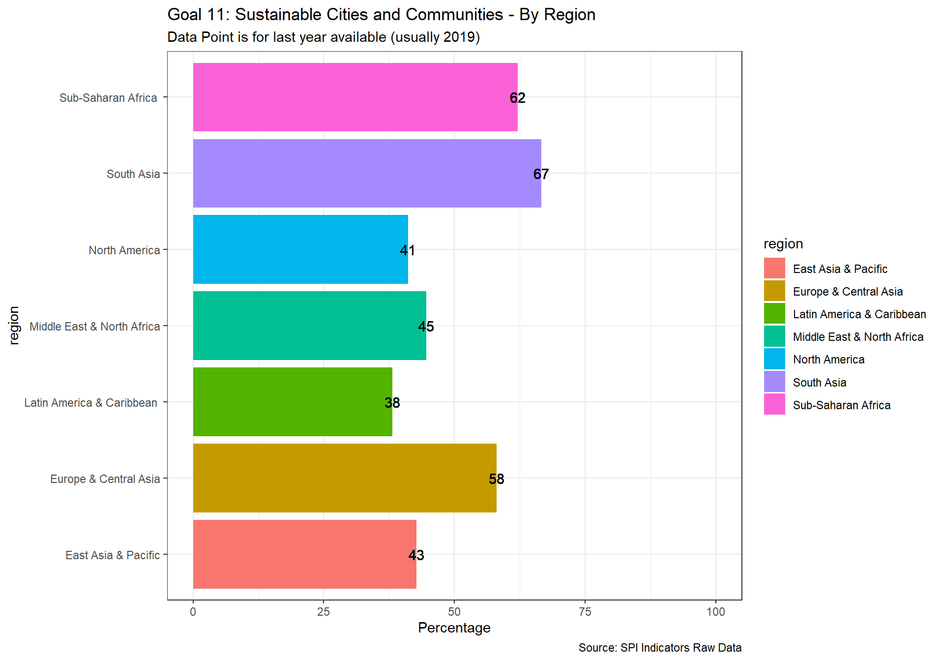
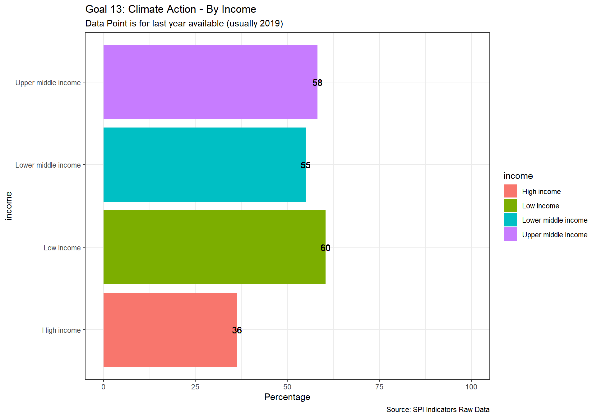
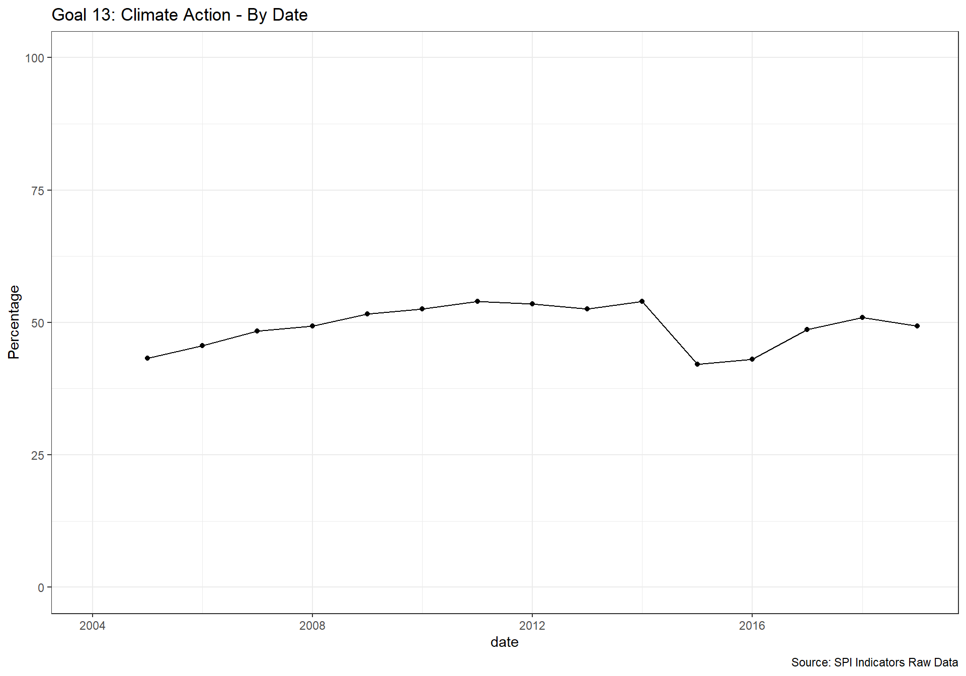
When we average over all indicators in a goal to get a score, we compute a 5 year moving average to avoid year to year variability in reporting for SDGs. The overall score for an SDG is then the 5 year average of the percentage of indicator values based on country, country data adjusted, or estimated or Global Monitoring data that were available for the SDG.
Because of the large data files and runtime of the program to calculate these indicators, the code to produce these indicators is in a separate file. https://github.com/stacybri/UN_Stats_SDG_Indicators_SPI/blob/master/02_programs/un_stats_cleaning.Rmd
2.3.2 Indicators 3.1 - 3.17
un_sdg_df <- read_csv(paste(raw_dir,'/3_DP/SPI_D3_UNSD_data_',window,'yr.csv',sep="")) %>%
rename(SPI.D3.1.POV = SPI.D3.1,
SPI.D3.2.HNGR = SPI.D3.2,
SPI.D3.3.HLTH = SPI.D3.3,
SPI.D3.4.EDUC = SPI.D3.4,
SPI.D3.5.GEND = SPI.D3.5,
SPI.D3.6.WTRS = SPI.D3.6,
SPI.D3.7.ENRG = SPI.D3.7,
SPI.D3.8.WORK = SPI.D3.8,
SPI.D3.9.INDY = SPI.D3.9,
SPI.D3.10.NEQL = SPI.D3.10,
SPI.D3.11.CITY = SPI.D3.11,
SPI.D3.12.CNSP = SPI.D3.12,
SPI.D3.13.CLMT = SPI.D3.13,
SPI.D3.14.LFWT = SPI.D3.14,
SPI.D3.15.LAND = SPI.D3.15,
SPI.D3.16.INST = SPI.D3.16,
SPI.D3.17.PTNS = SPI.D3.17
) %>%
select(country, date, starts_with("SPI")) %>%
select(-SPI.D3.14.LFWT)
#add to spi databases
spi_df <- spi_df %>%
left_join(un_sdg_df)
#map the values
un_sdg_map <- un_sdg_df %>%
select(country, date, starts_with("SPI"))
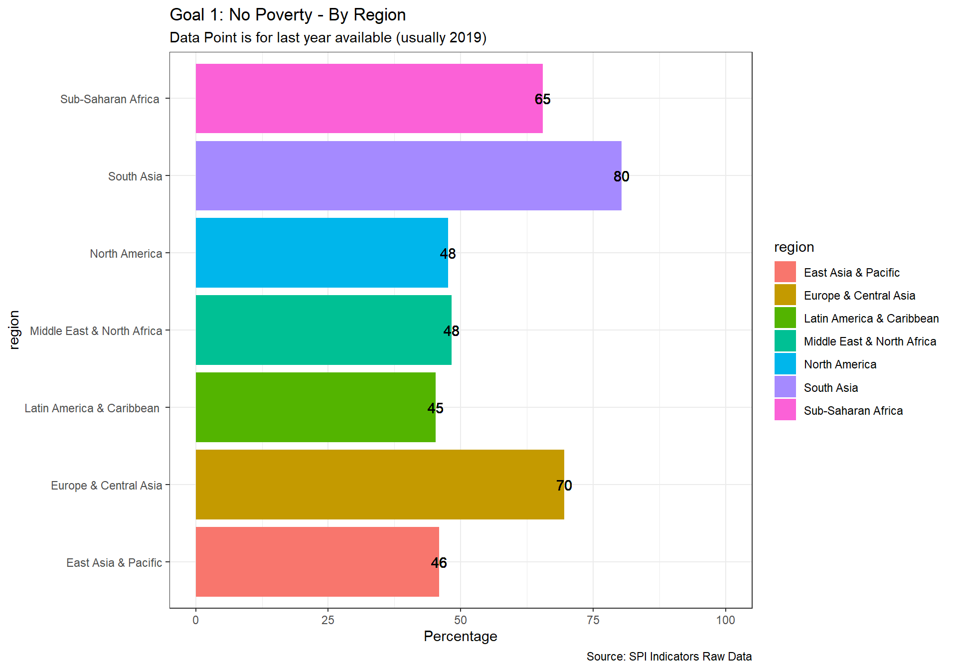
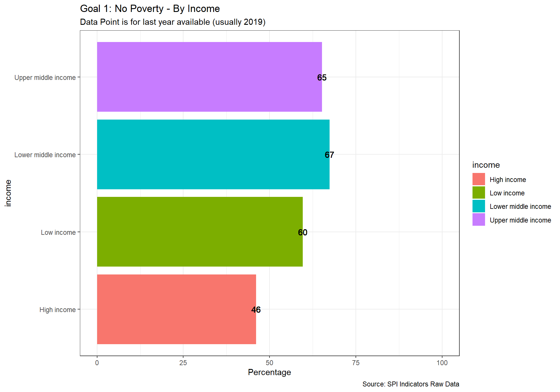
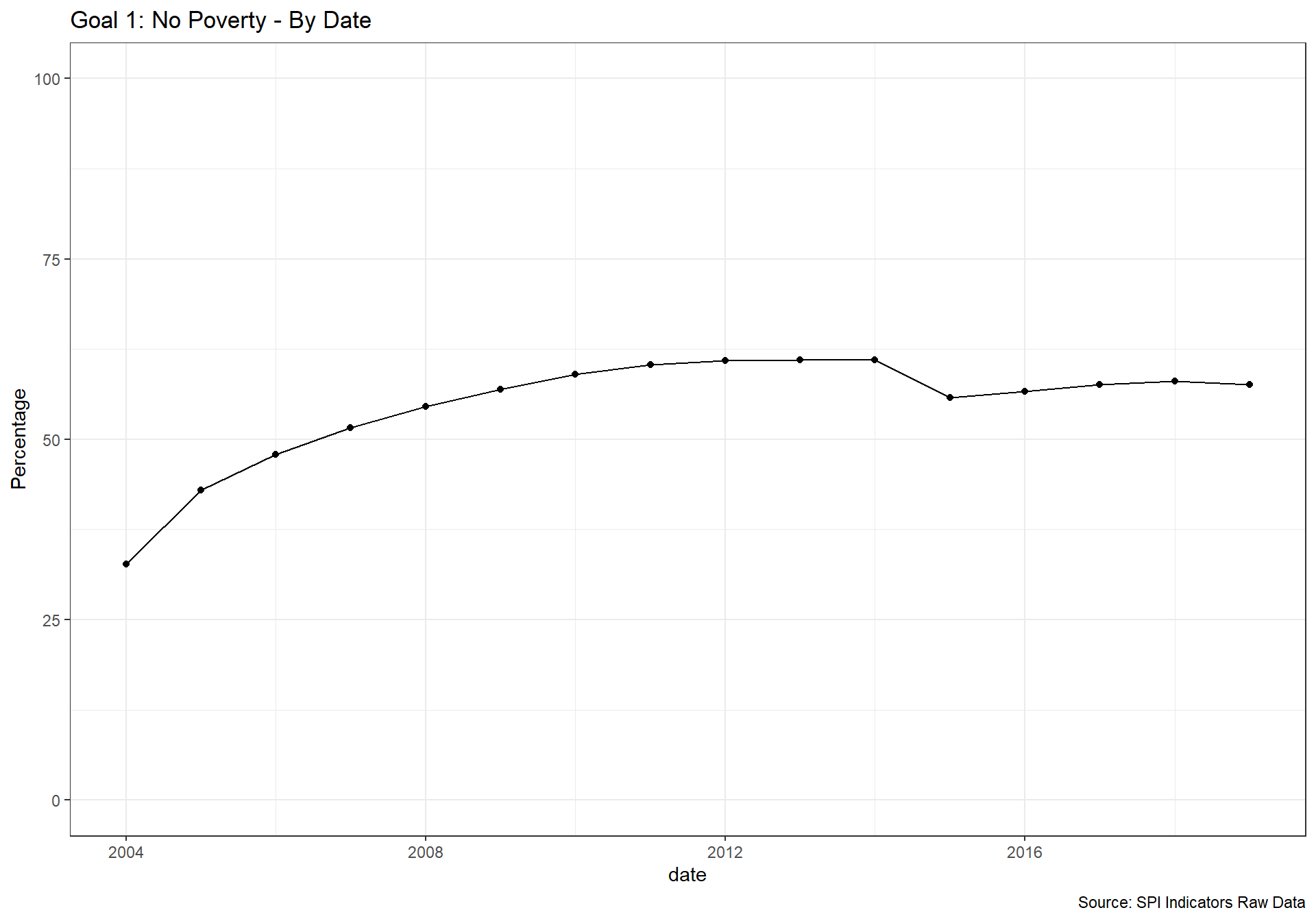
spi_mapper('un_sdg_map','SPI.D3.1.POV','Goal 1: No Poverty')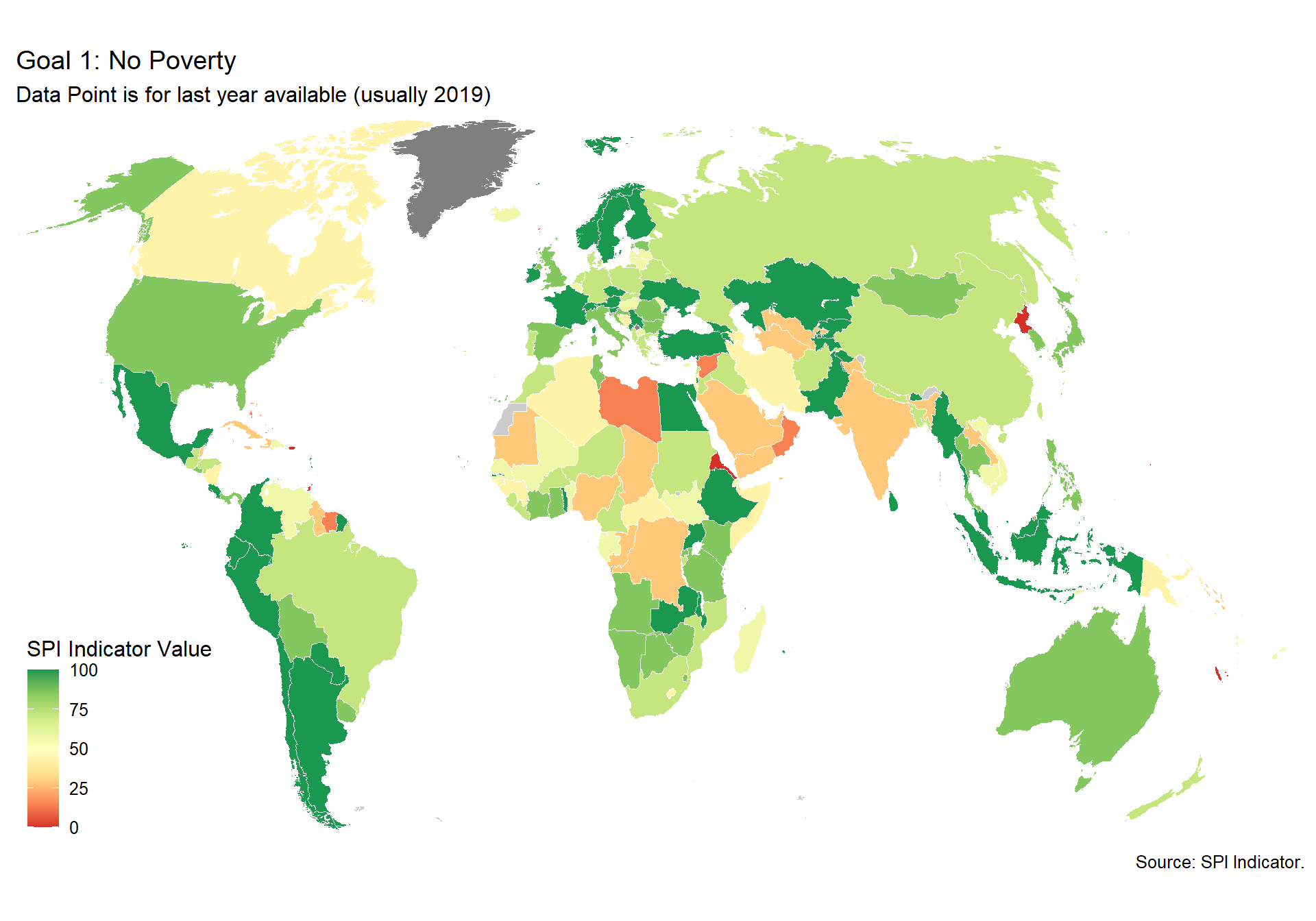
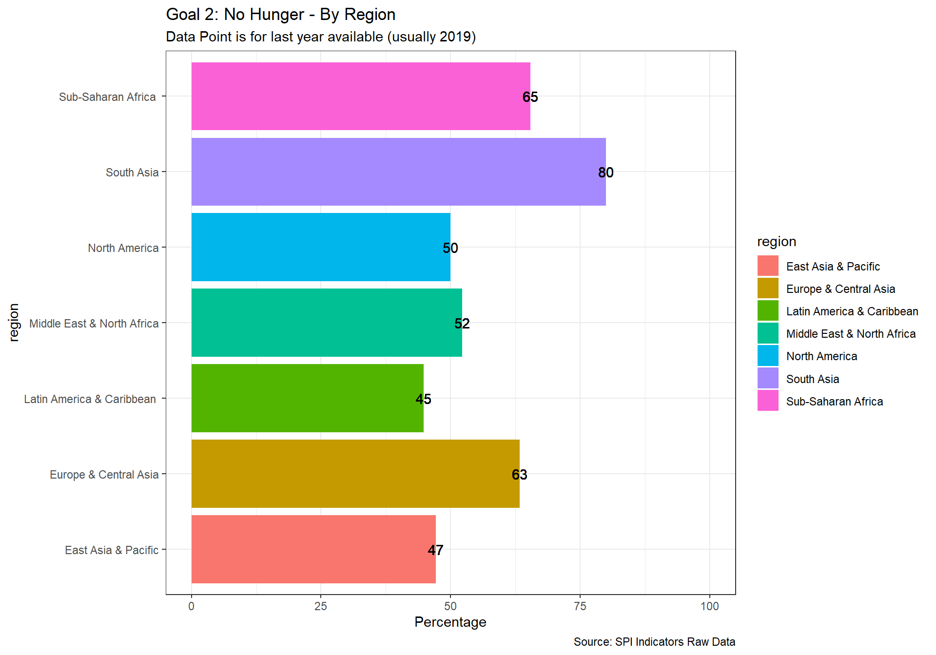
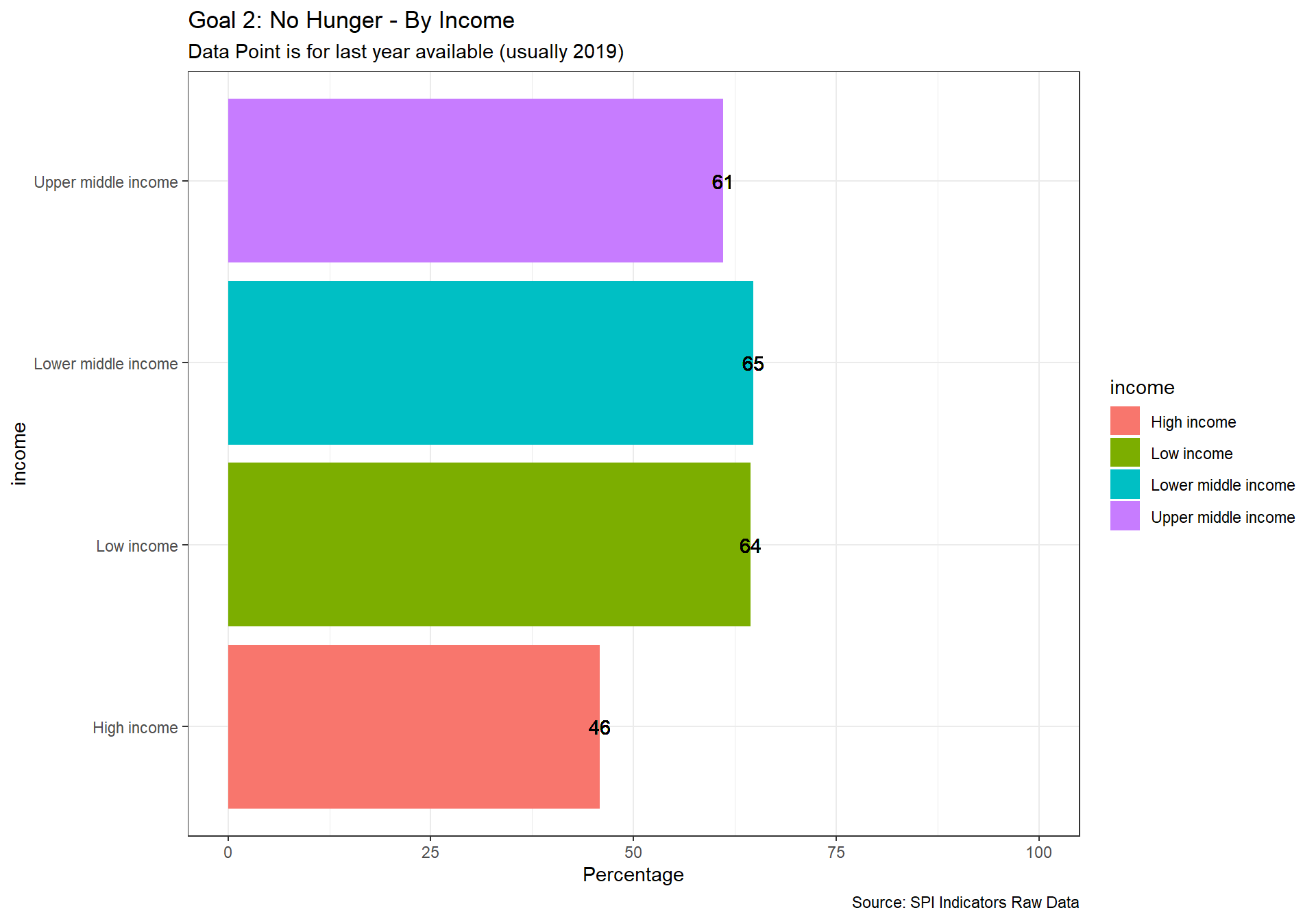
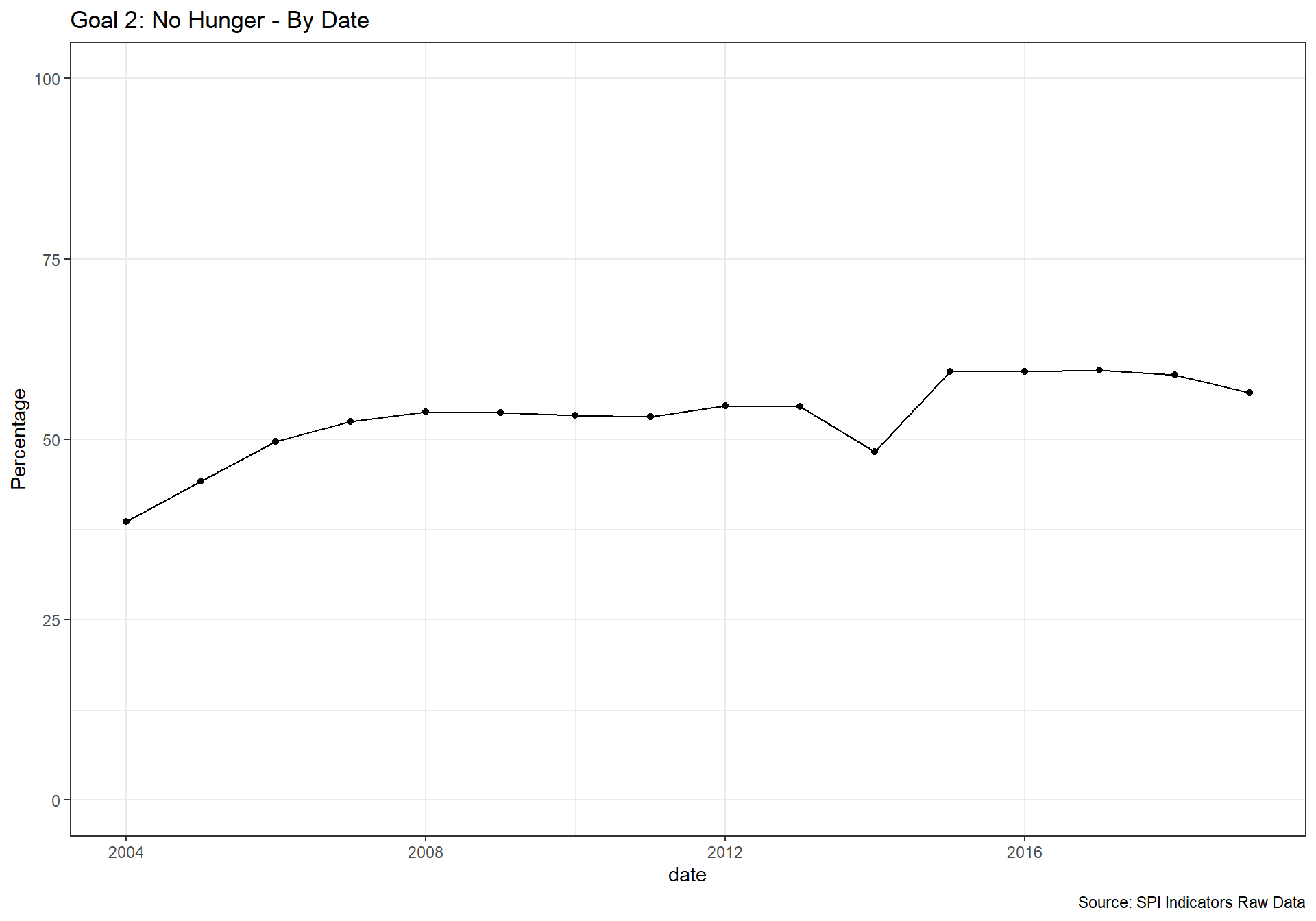
spi_mapper('un_sdg_map','SPI.D3.2.HNGR','Goal 2: No Hunger')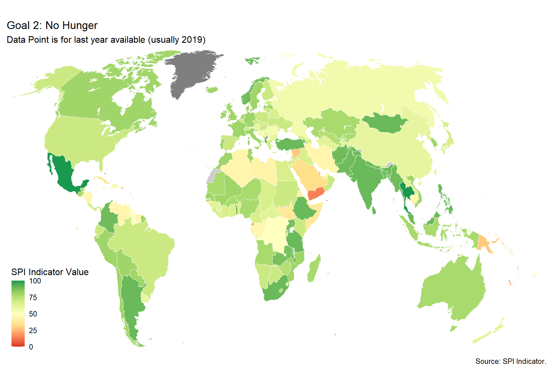
spi_mapper('un_sdg_map','SPI.D3.3.HLTH','Goal 3: Good Health and Well-being')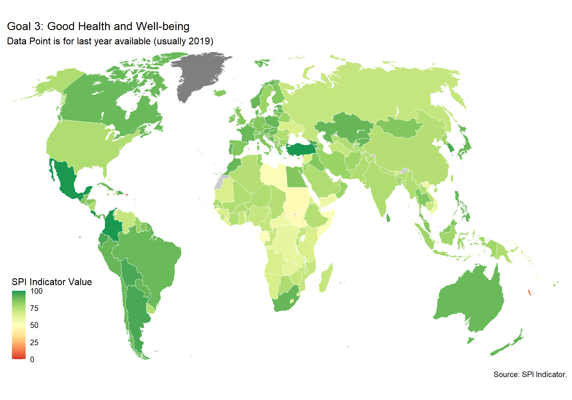
spi_mapper('un_sdg_map','SPI.D3.4.EDUC','Goal 4: Quality Education ')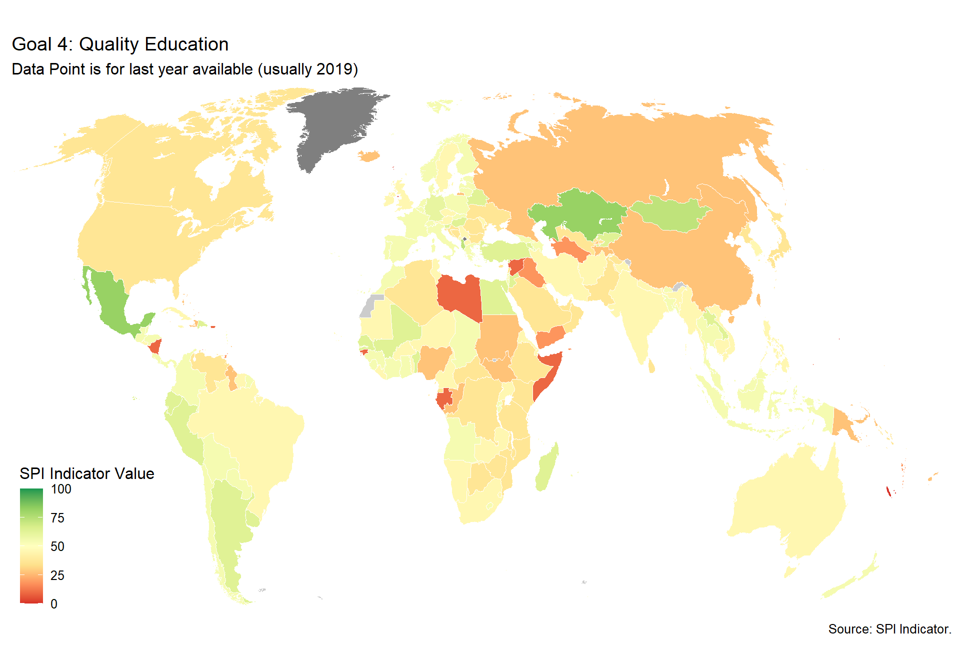
spi_mapper('un_sdg_map','SPI.D3.5.GEND','Goal 5: Gender Equality ')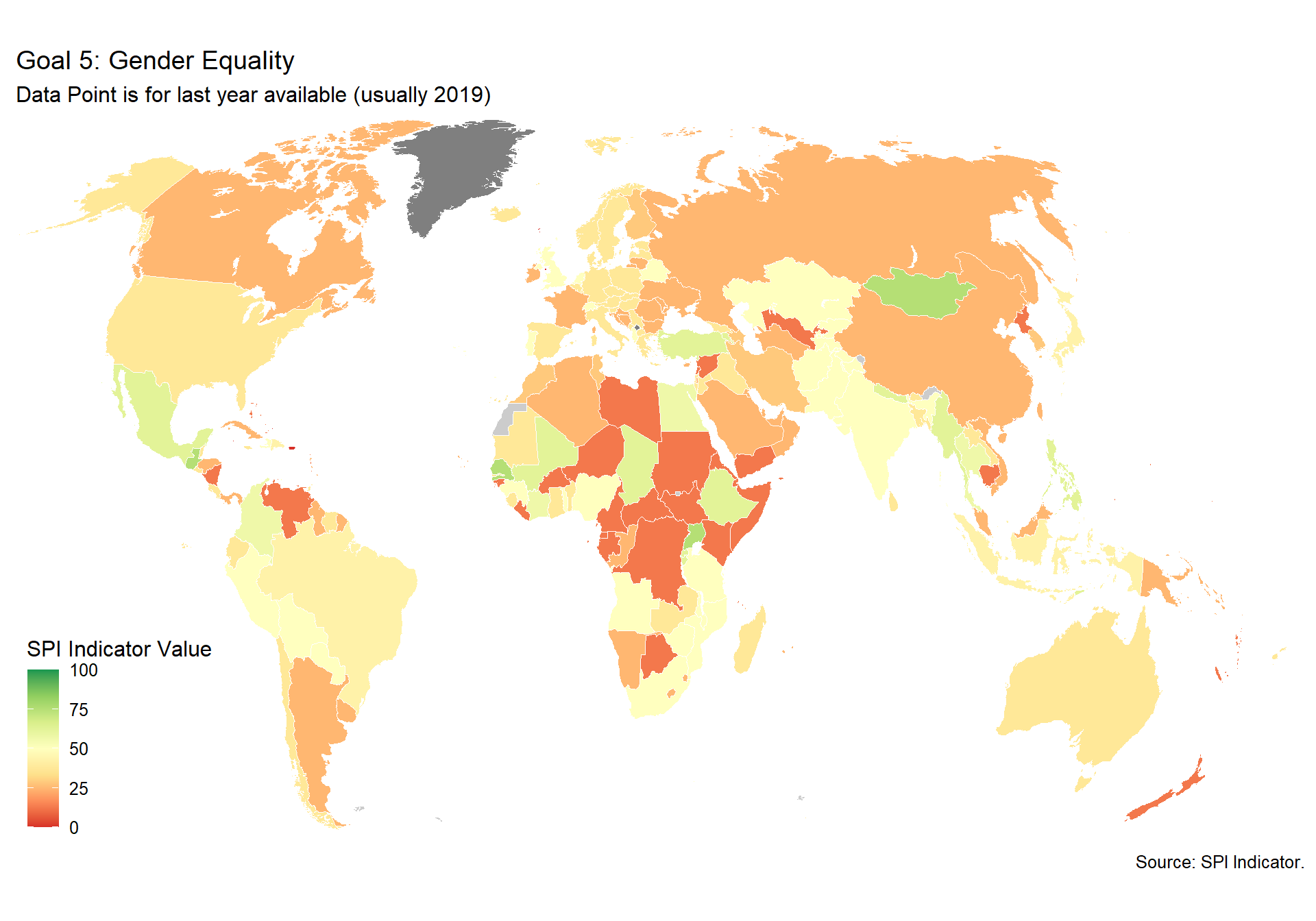
spi_mapper('un_sdg_map','SPI.D3.6.WTRS','Goal 6: Clean Water and Sanitation ')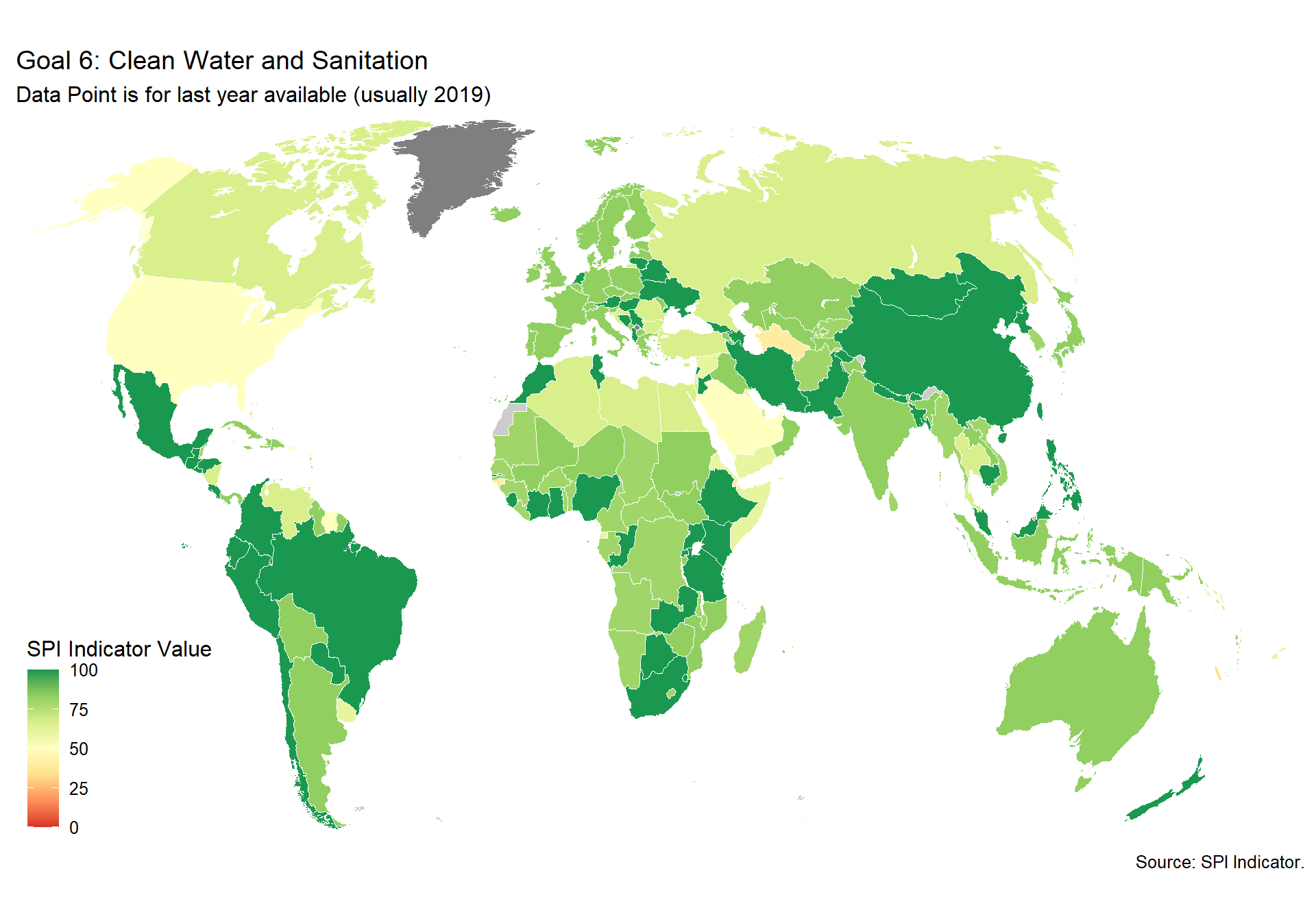
spi_mapper('un_sdg_map','SPI.D3.7.ENRG','Goal 7: Affordable and Clean Energy')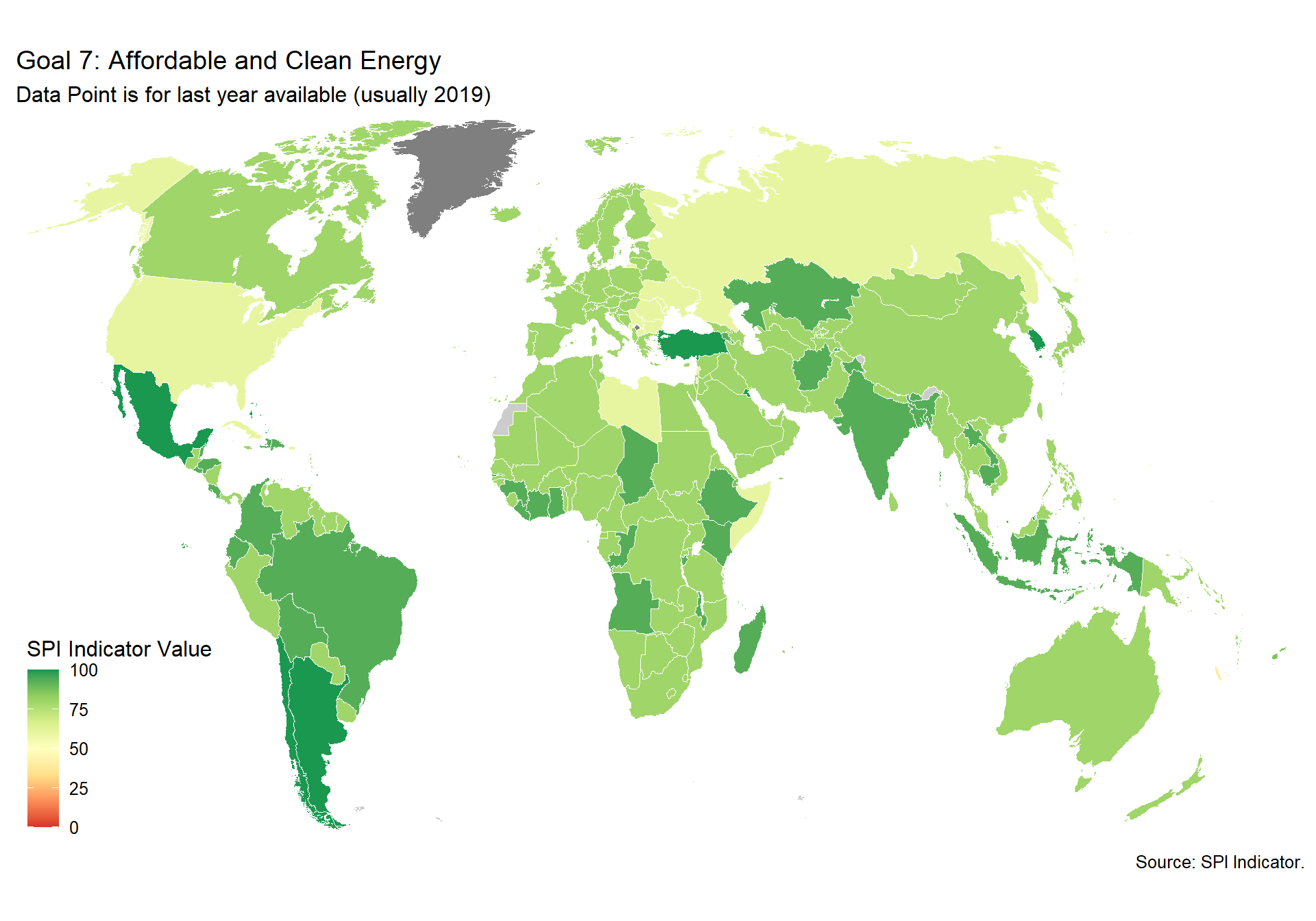
spi_mapper('un_sdg_map','SPI.D3.8.WORK','Goal 8: Decent Work and Economic Growth ')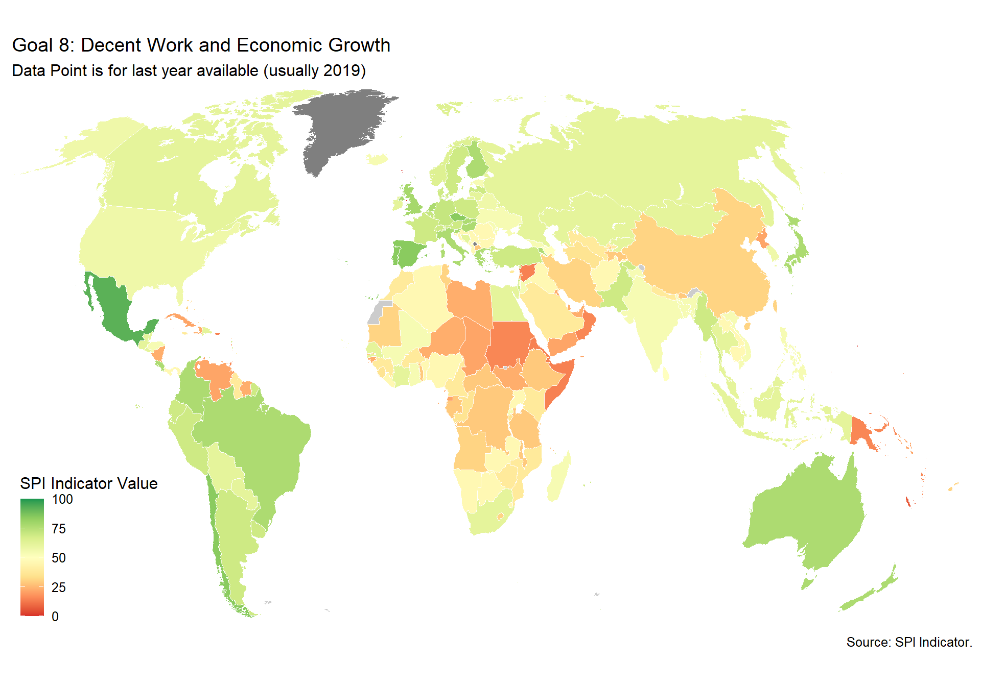
spi_mapper('un_sdg_map','SPI.D3.9.INDY','Goal 9: Industry, Innovation and Infrastructure ')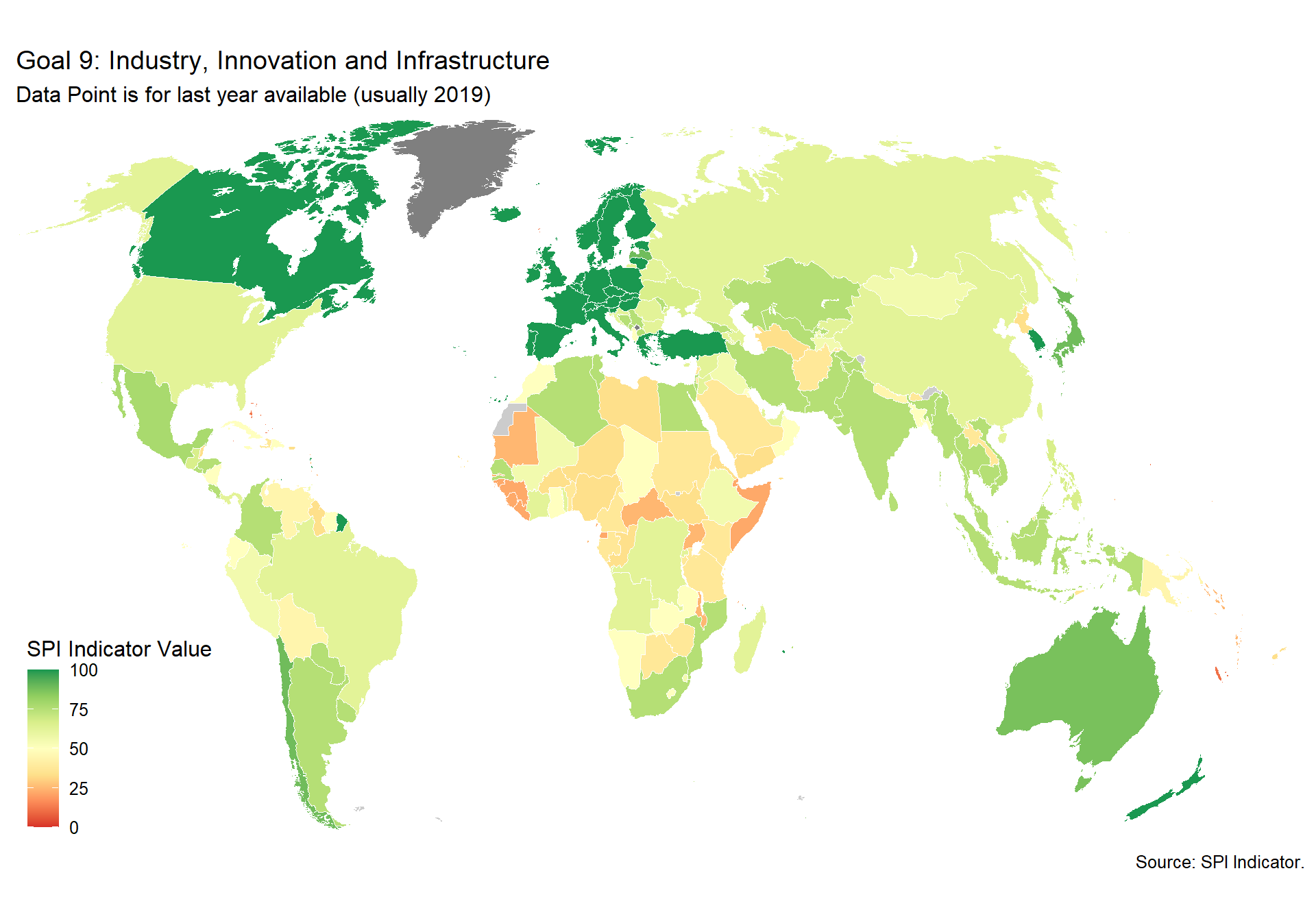
spi_mapper('un_sdg_map','SPI.D3.10.NEQL','Goal 10: Reduced Inequality ')
spi_mapper('un_sdg_map','SPI.D3.11.CITY','Goal 11: Sustainable Cities and Communities')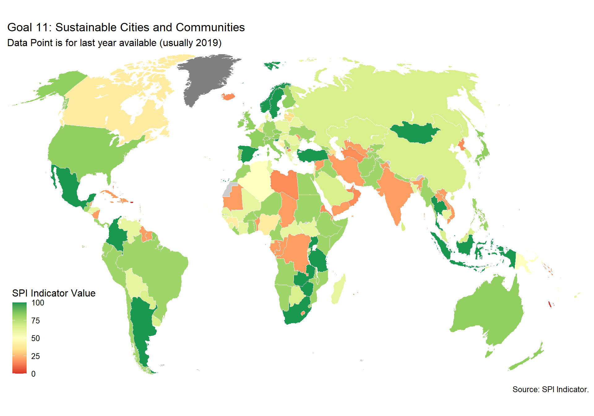
spi_mapper('un_sdg_map','SPI.D3.12.CNSP','Goal 12: Responsible Consumption and Production ')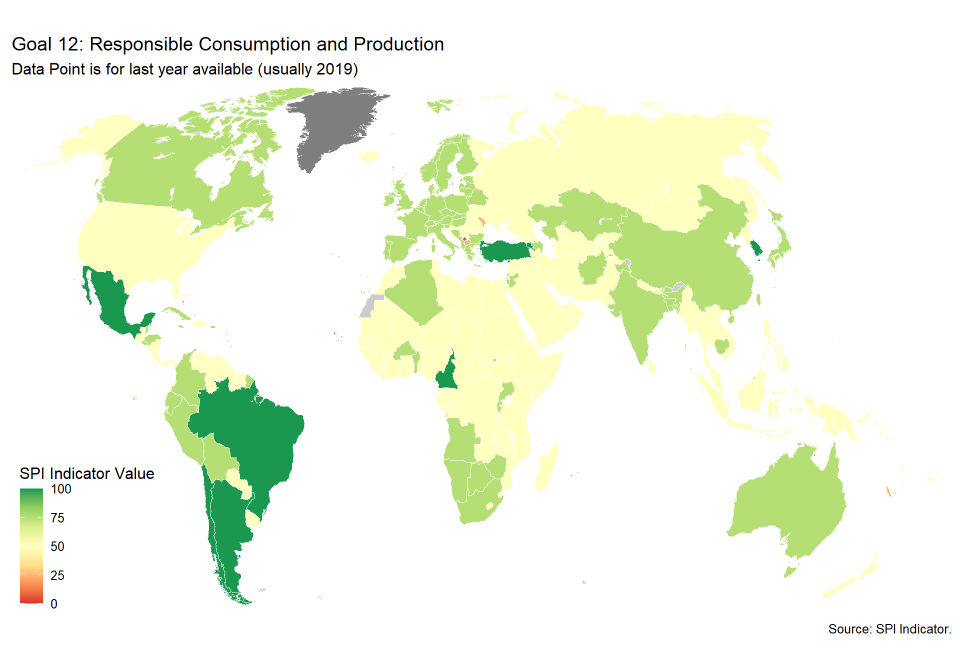
spi_mapper('un_sdg_map','SPI.D3.13.CLMT','Goal 13: Climate Action')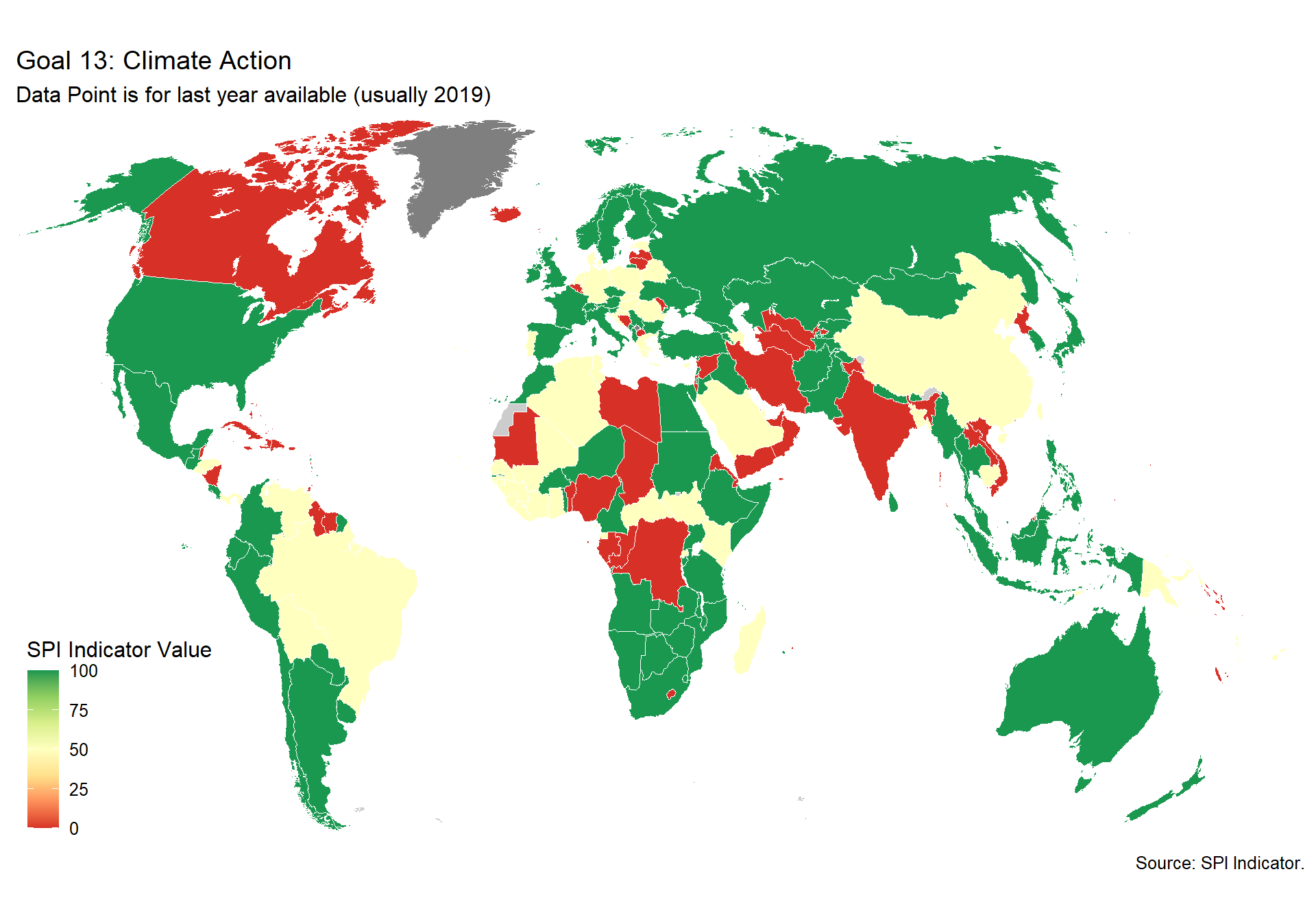
#spi_mapper('un_sdg_map','SPI.D3.14.LFWT','Goal 14: Life Below Water')
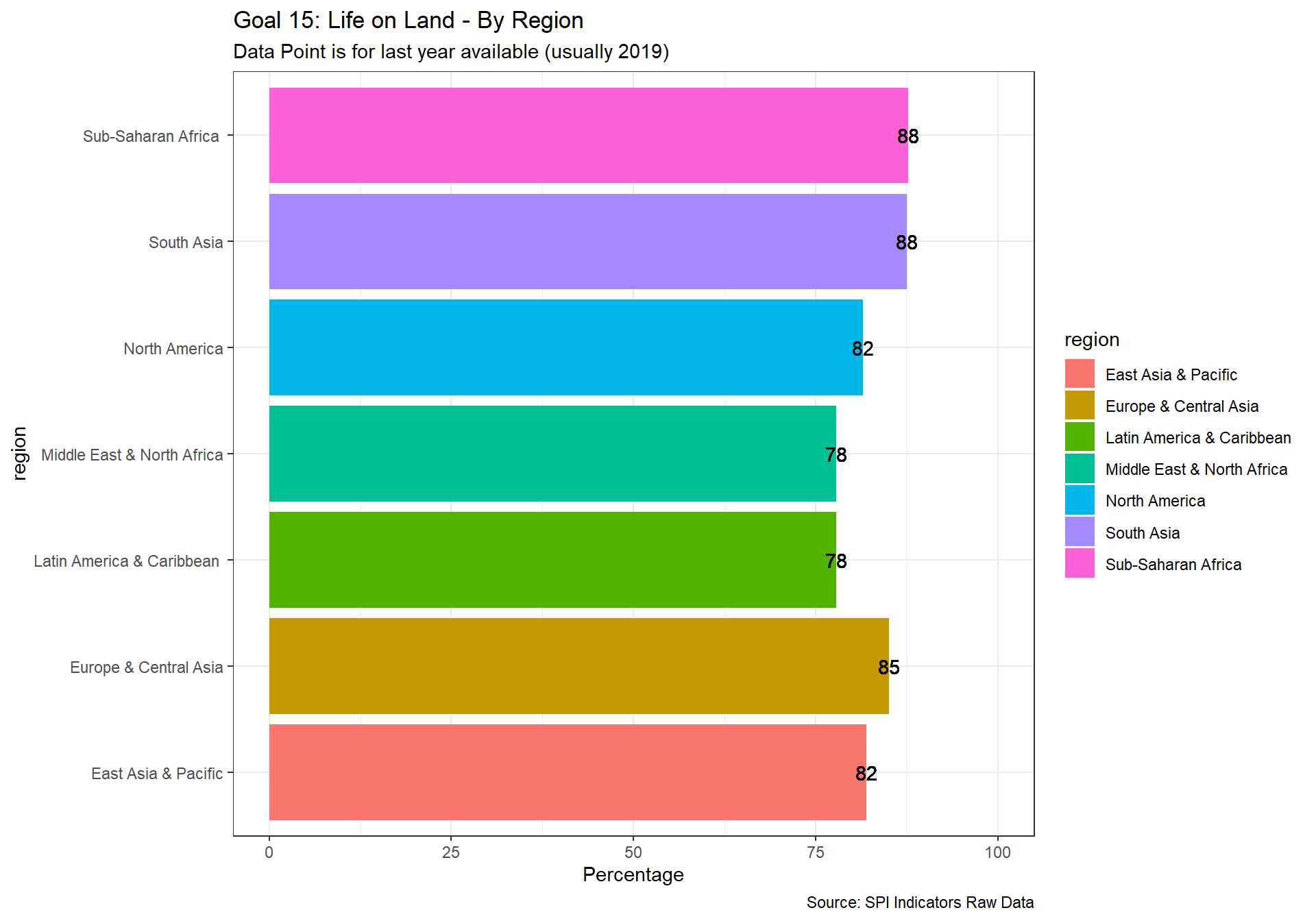
spi_mapper('un_sdg_map','SPI.D3.15.LAND','Goal 15: Life on Land')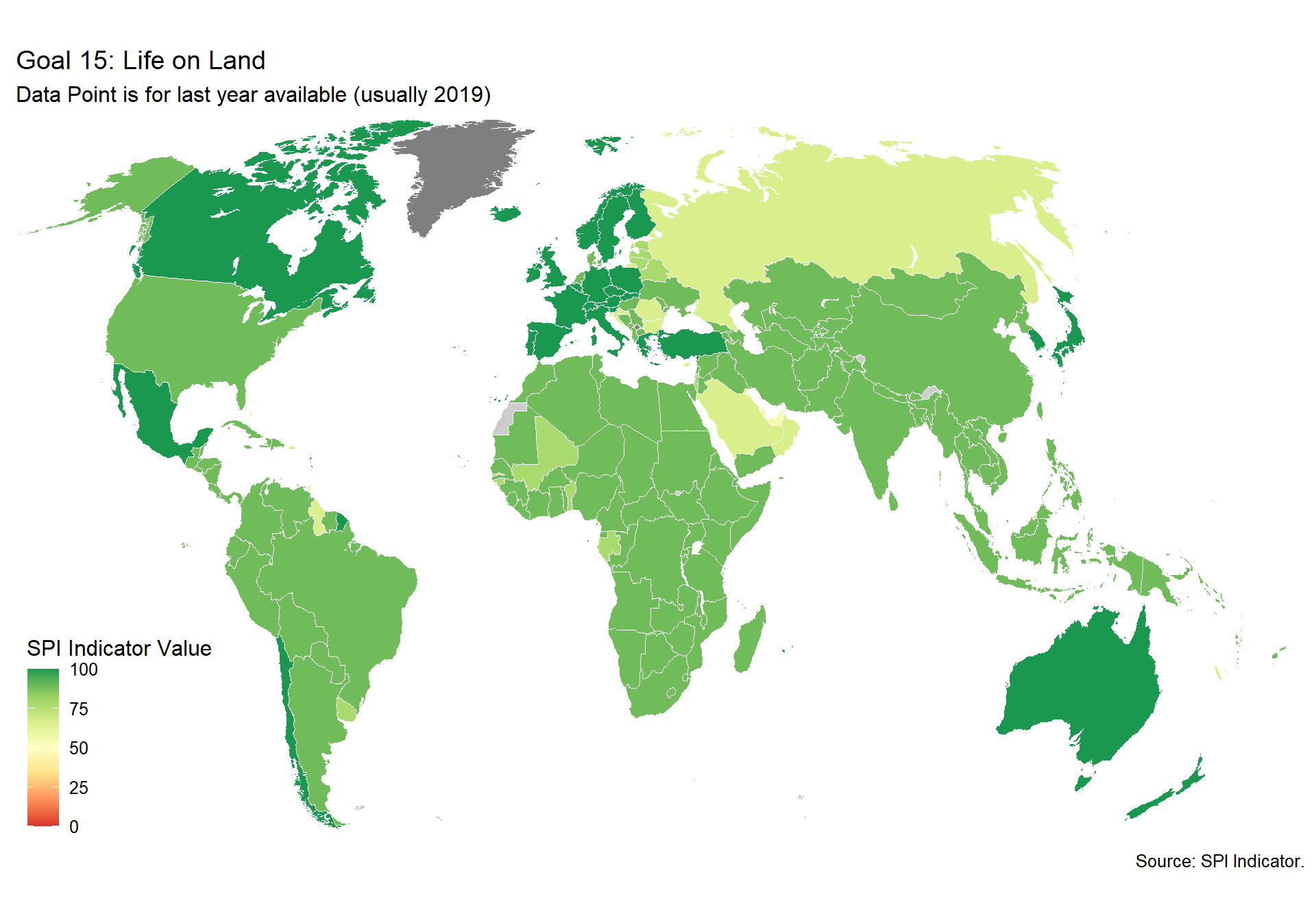
spi_mapper('un_sdg_map','SPI.D3.16.INST','Goal 16: Peace and Justice Strong Institutions')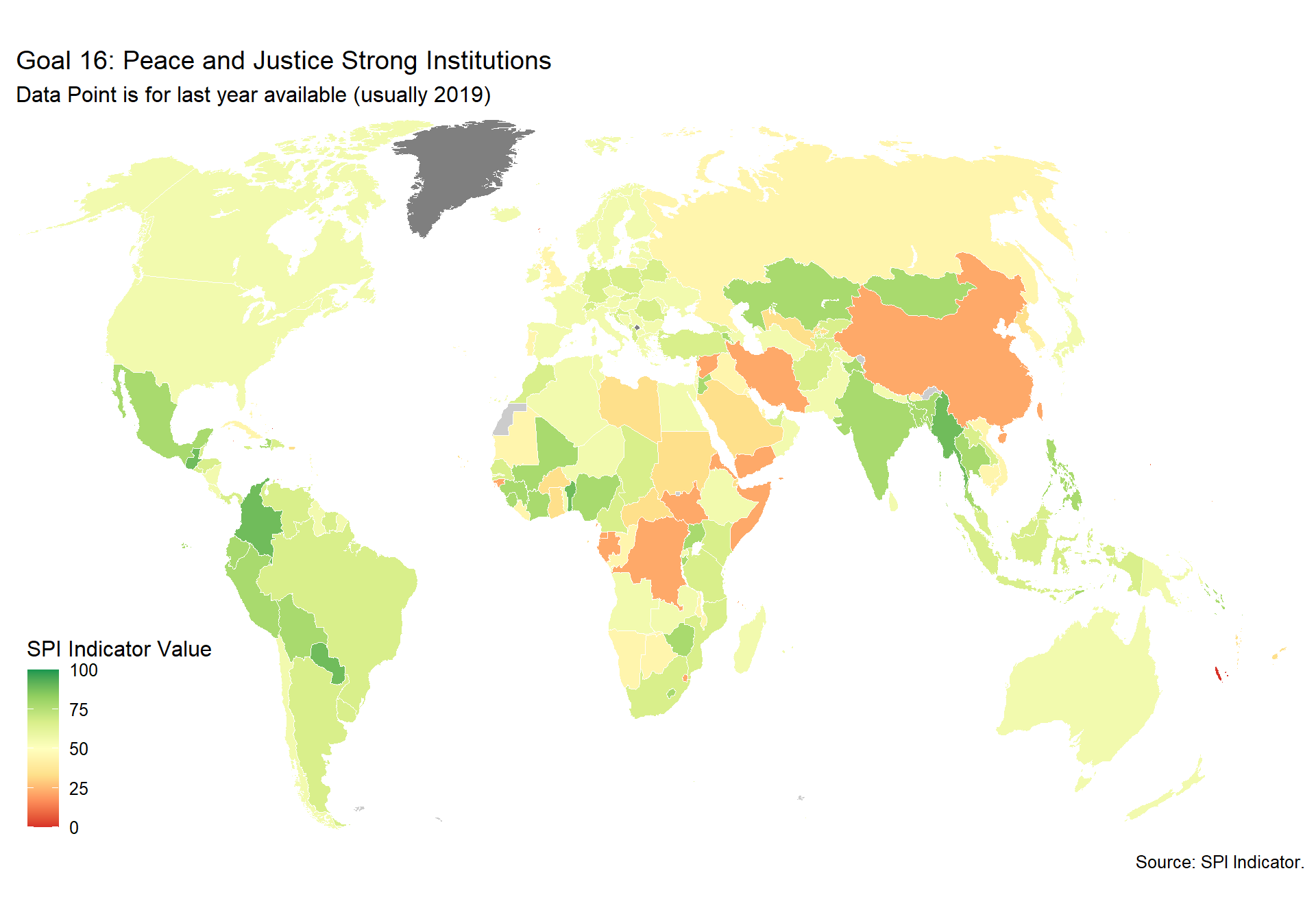
spi_mapper('un_sdg_map','SPI.D3.17.PTNS','Goal 17: Partnerships to achieve the Goal ')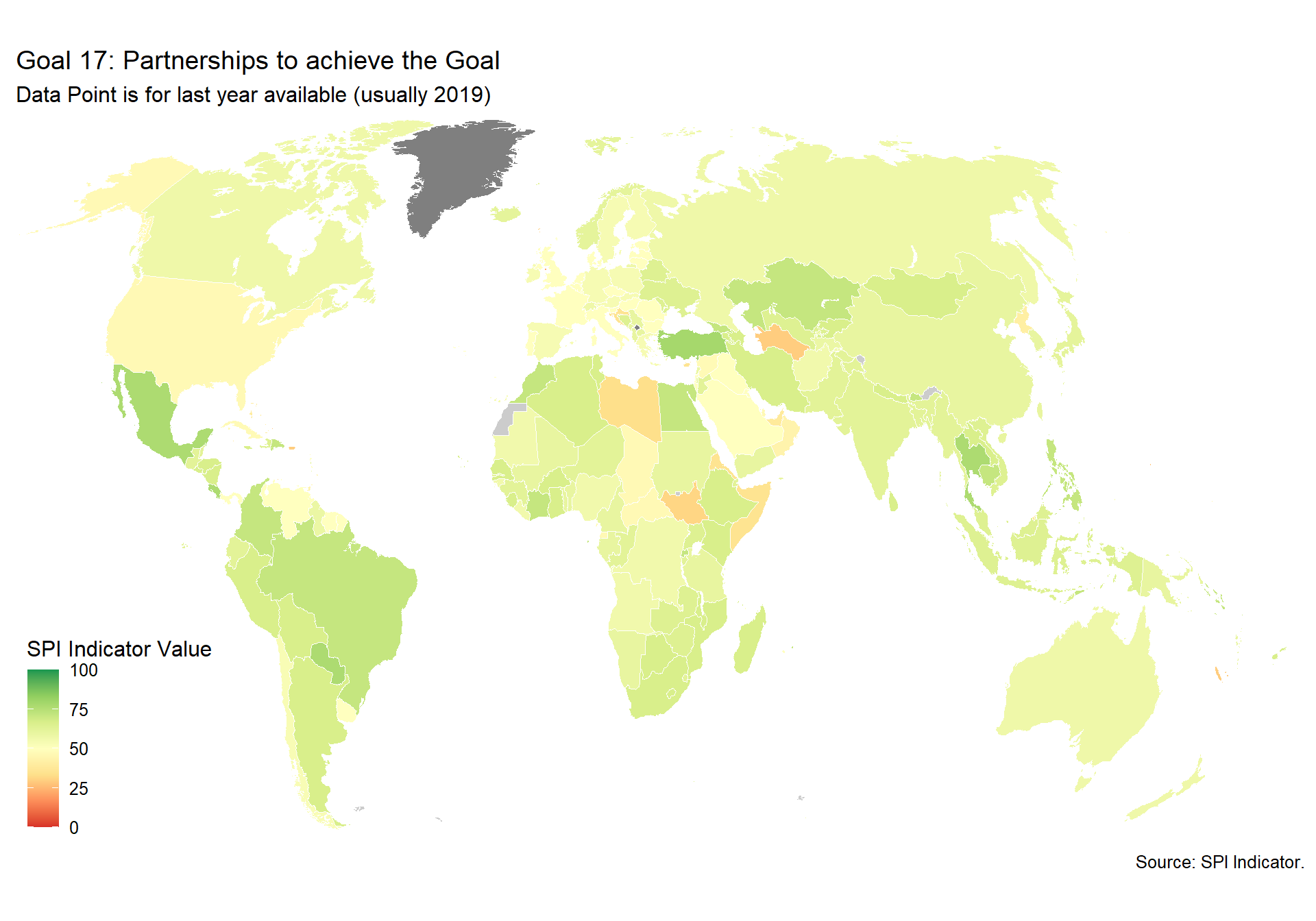
2.4 Data Sources
Cleaning for the Data Sources Indicators. Data Sources (4 Indicators):
- 4.1_SOCS - Indicator 4.1: censuses and surveys
- 4.2_SOAD - Indicator 4.2: administrative data
- 4.3_SOGS - Indicator 4.3: geospatial data
- 4.4_SOPC - Indicator 4.4: private/citizen generated data
2.4.1 Indicator 4.1: censuses and surveys
This indicator draws from data collected by the Statistical Performance Indicators team. The following censuses and surveys are considered:
- Population & Housing census
- Agriculture census
- Business/establishment census
- Household Survey on income/ consumption/ expenditure/ budget/ Integrated Survey
- Agriculture survey
- Labor Force Survey
- Health/Demographic survey
- Business/establishment survey
2.4.1.1 Scoring details
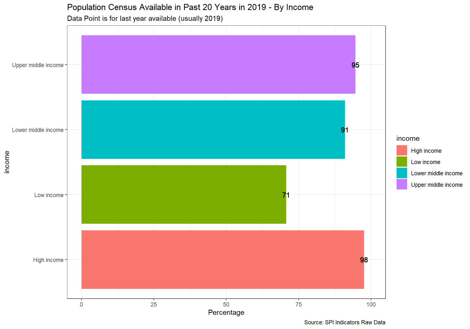
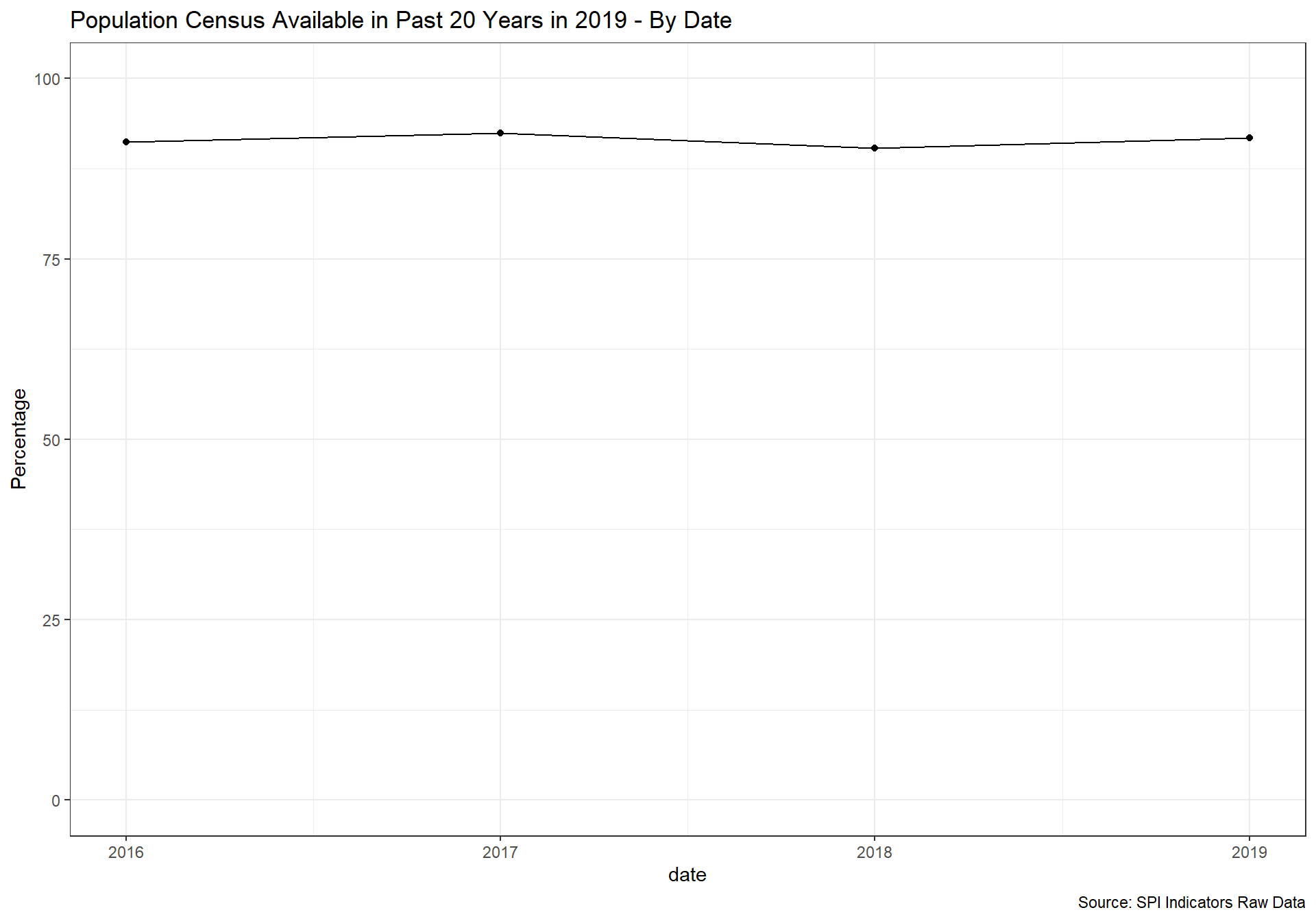
2.4.1.1.1 Population & Housing census
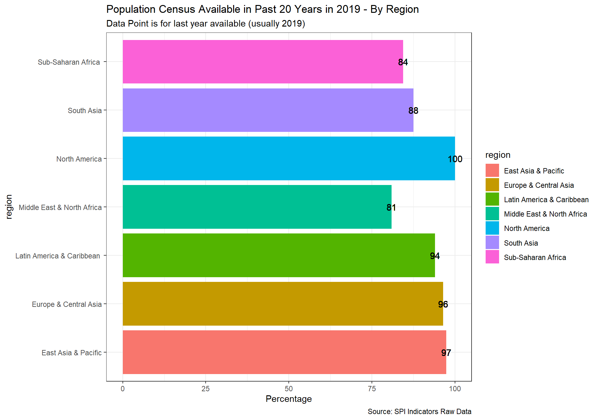
Population censuses collect data on the size, distribution and composition of population and information on a broad range of social and economic characteristics of the population. It also provides sampling frames for household and other surveys. Housing censuses provide information on the supply of housing units, the structural characteristics and facilities, and health and the development of normal family living conditions. Data obtained as part of the population census, including data on homeless persons, are often used in the presentation and analysis of the results of the housing census. It is recommended that population and housing censuses be conducted at least every 10 years.
1 Point. Population census done within last 10 years
0.5 Points. Population census done within last 20 years
0 Points. Otherwise
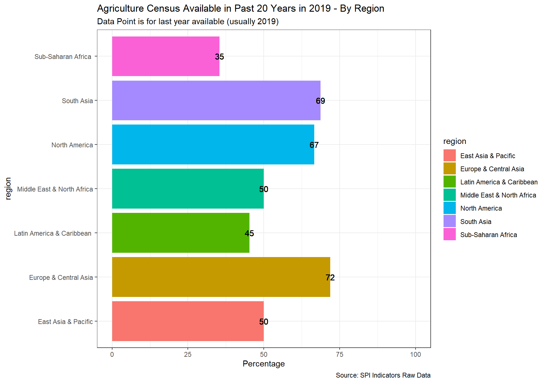
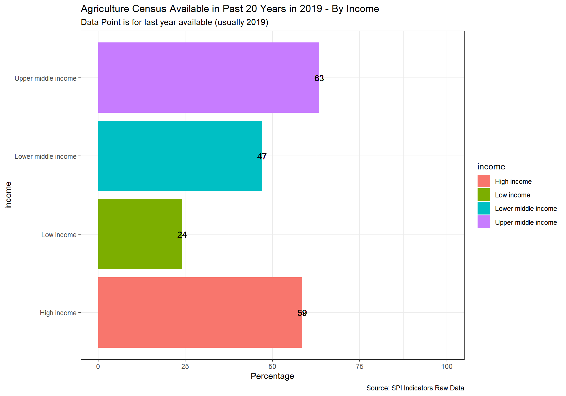
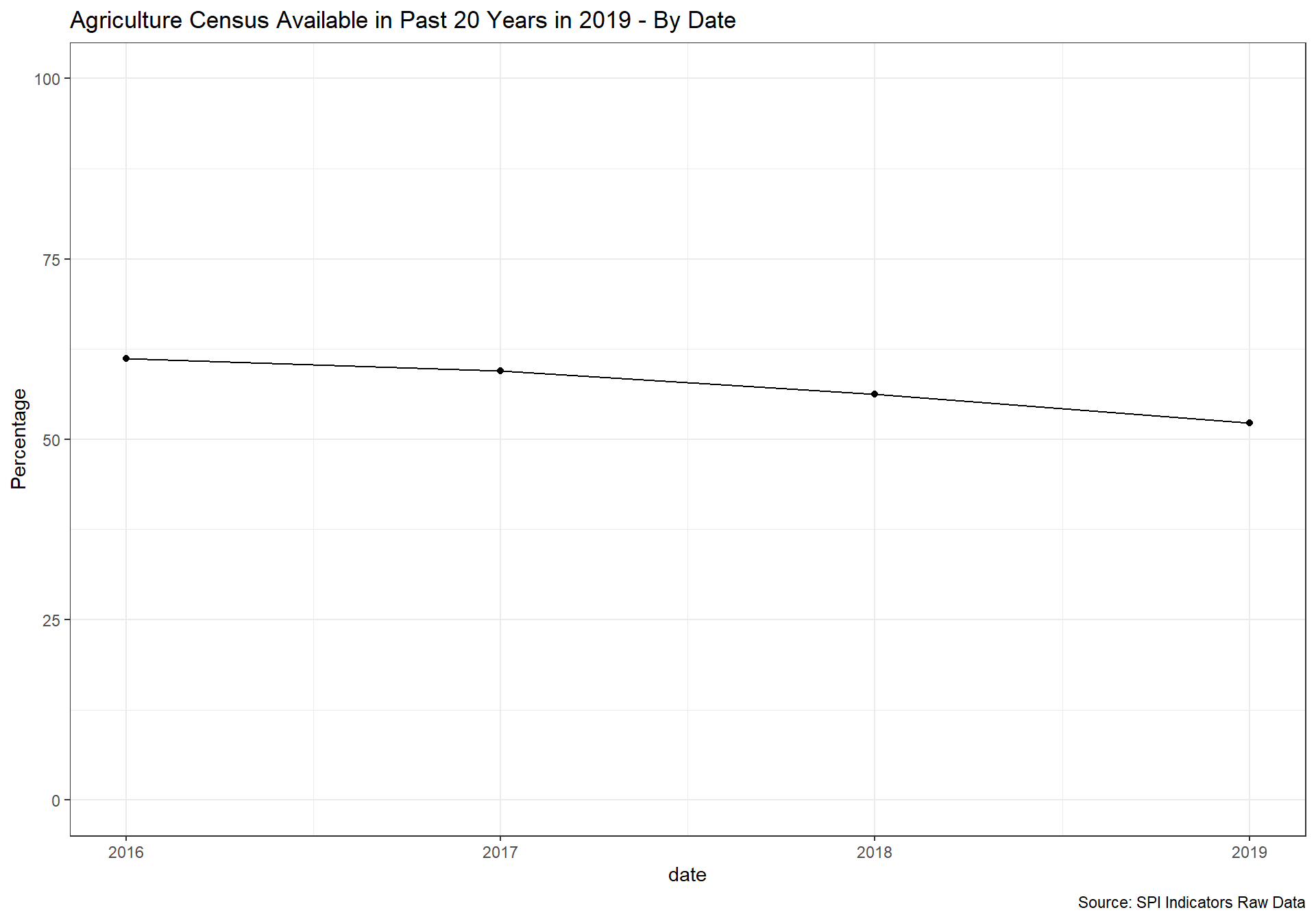
2.4.1.1.2 Agriculture census
Agriculture censuses collect information on agricultural activities, such as size of holding, land tenure, land use, employment and production, and provide basic structural data and sampling frames for agricultural surveys. Censuses of agriculture normally involves collecting key structural data by complete enumeration of all agricultural holdings, in combination with more detailed structural data using sampling methods. It is recommended that agricultural censuses be conducted at least every 10 years.
1 Point. census done within last 10 years
0.5 Points. census done within last 20 years
0 Points. Otherwise
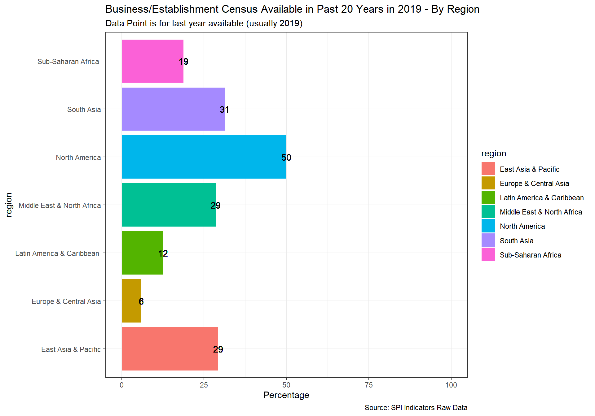
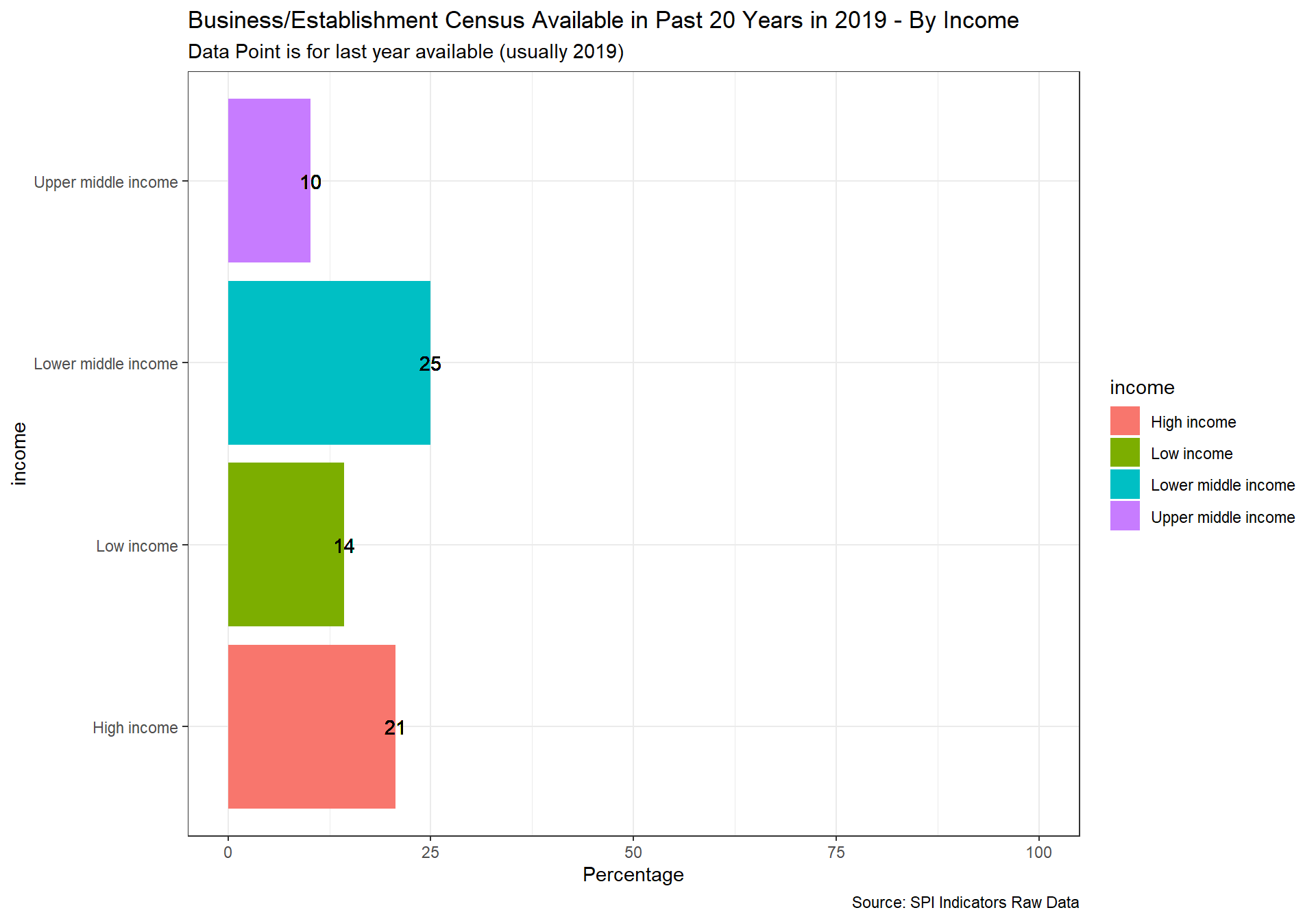
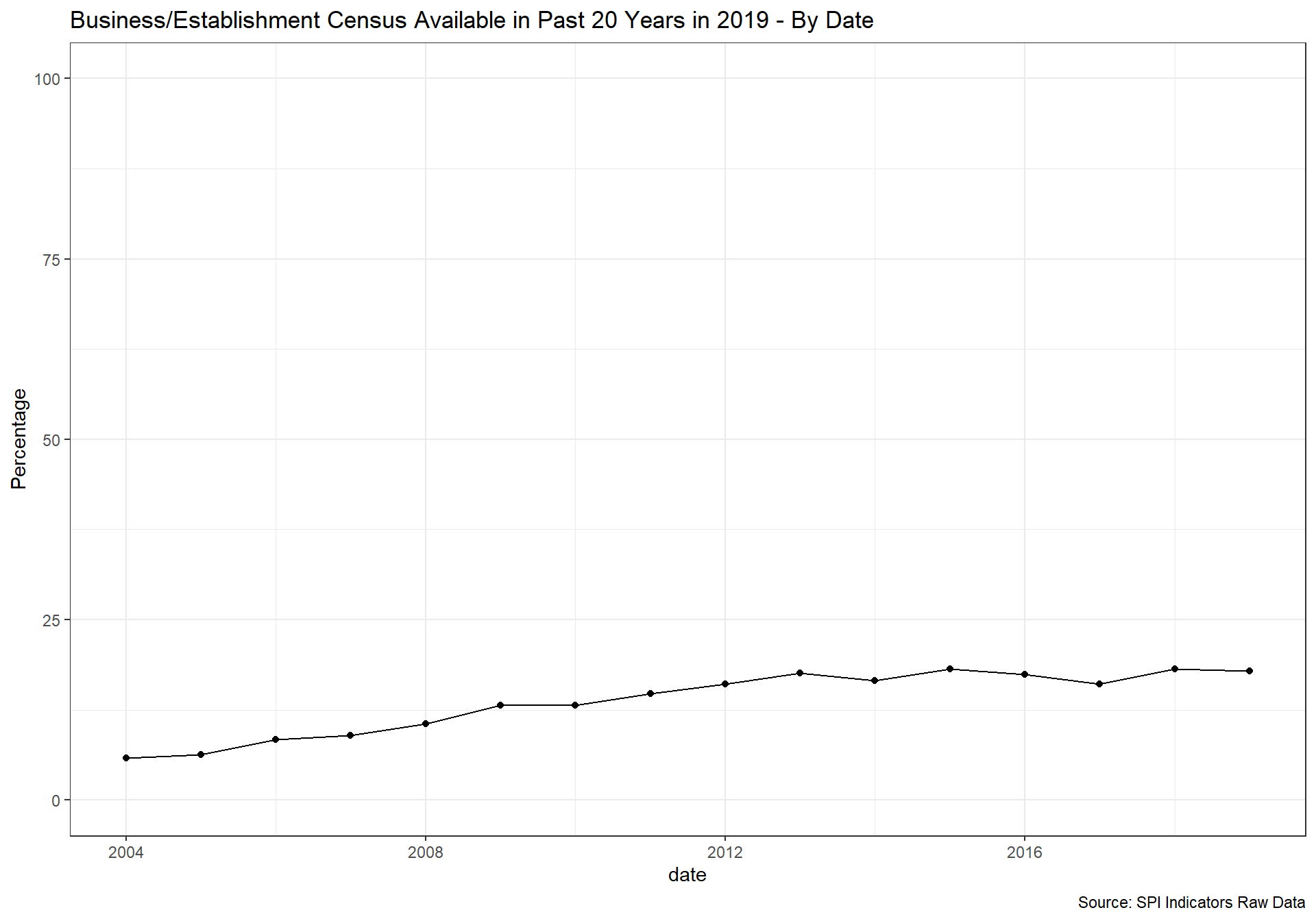
2.4.1.1.3 Business/establishment census
Business/establishment censuses provide valuable information on all economic activities, number of employed and size of establishments in the economy. Business Register information is establishment-based and includes business location, organization type (e.g. subsidiary or parent), industry classification, and operating data (e.g., receipts and employment).
1 Point. census done within last 10 years
0.5 Points. census done within last 20 years
0 Points. Otherwise
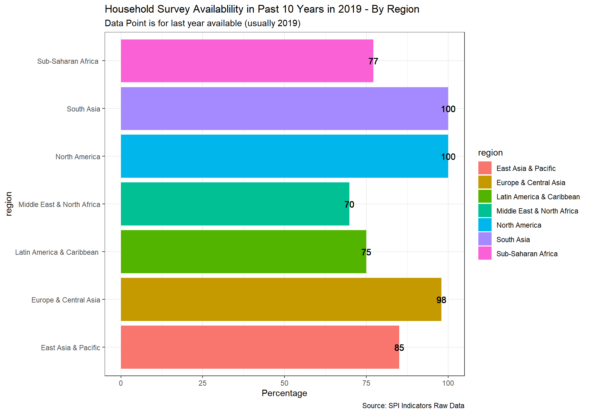
2.4.1.1.4 Household Survey on income/consumption/expenditure/budget/Integrated Survey
These surveys collect data on household income (including income in kind), consumption and expenditure. They typically include income, expenditure, and consumption surveys, household budget surveys, integrated surveys. It is recommended that surveys on income and expenditure be conducted at least every 3 to 5 years.
1 Point. 3 or more surveys done within past 10 years
0.67 Points. 2 surveys done within past 10 years;
0.33 Points. 1 survey done within past 10 years;
0 Points. None within past 10 years
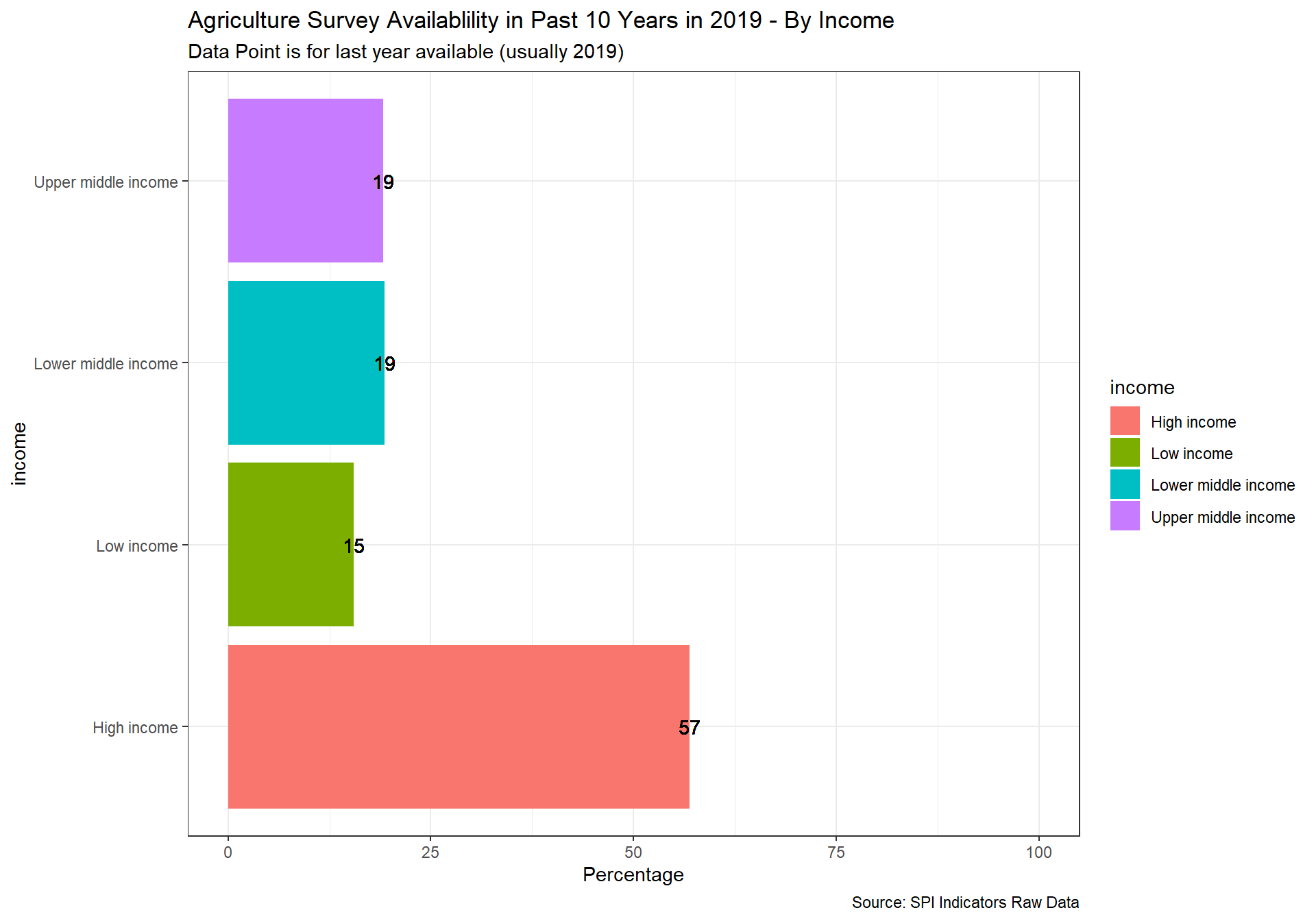
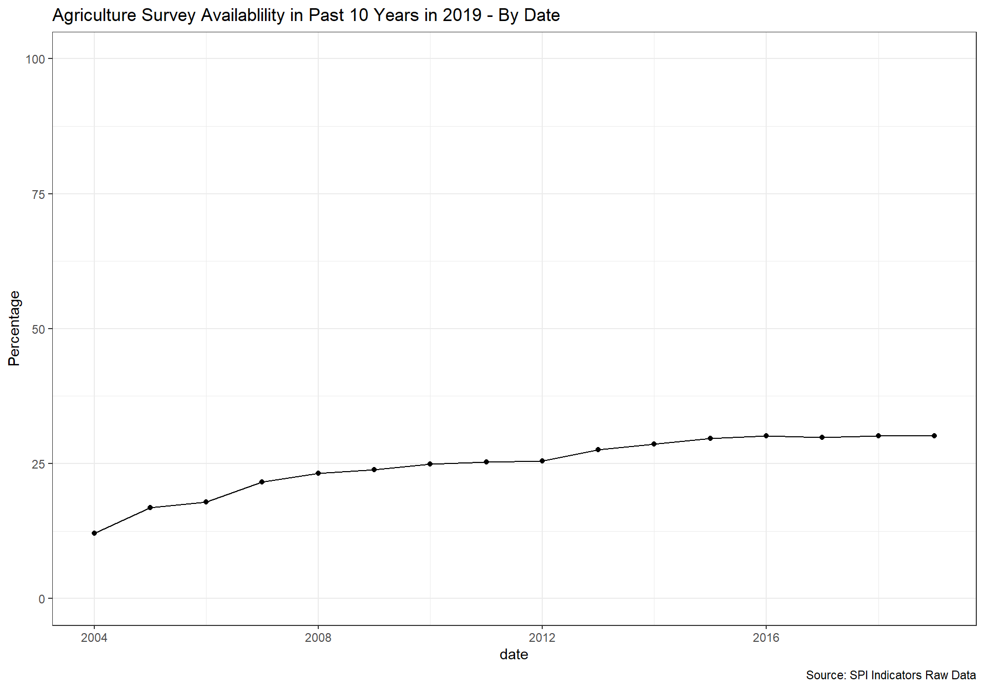
2.4.1.1.5 Agriculture survey
Agricultural surveys refer to surveys of agricultural holdings based on the sampling frames established by the agricultural census. These are surveys on agricultural land, production, crops and livestock, aquaculture, labor and cost, and time use. Some issues, such as gender and food security, are of interest to most agriculture surveys.
1 Point. 3 or more surveys done within past 10 years
0.67 Points. 2 surveys done within past 10 years;
0.33 Points. 1 survey done within past 10 years;
0 Points. None within past 10 years
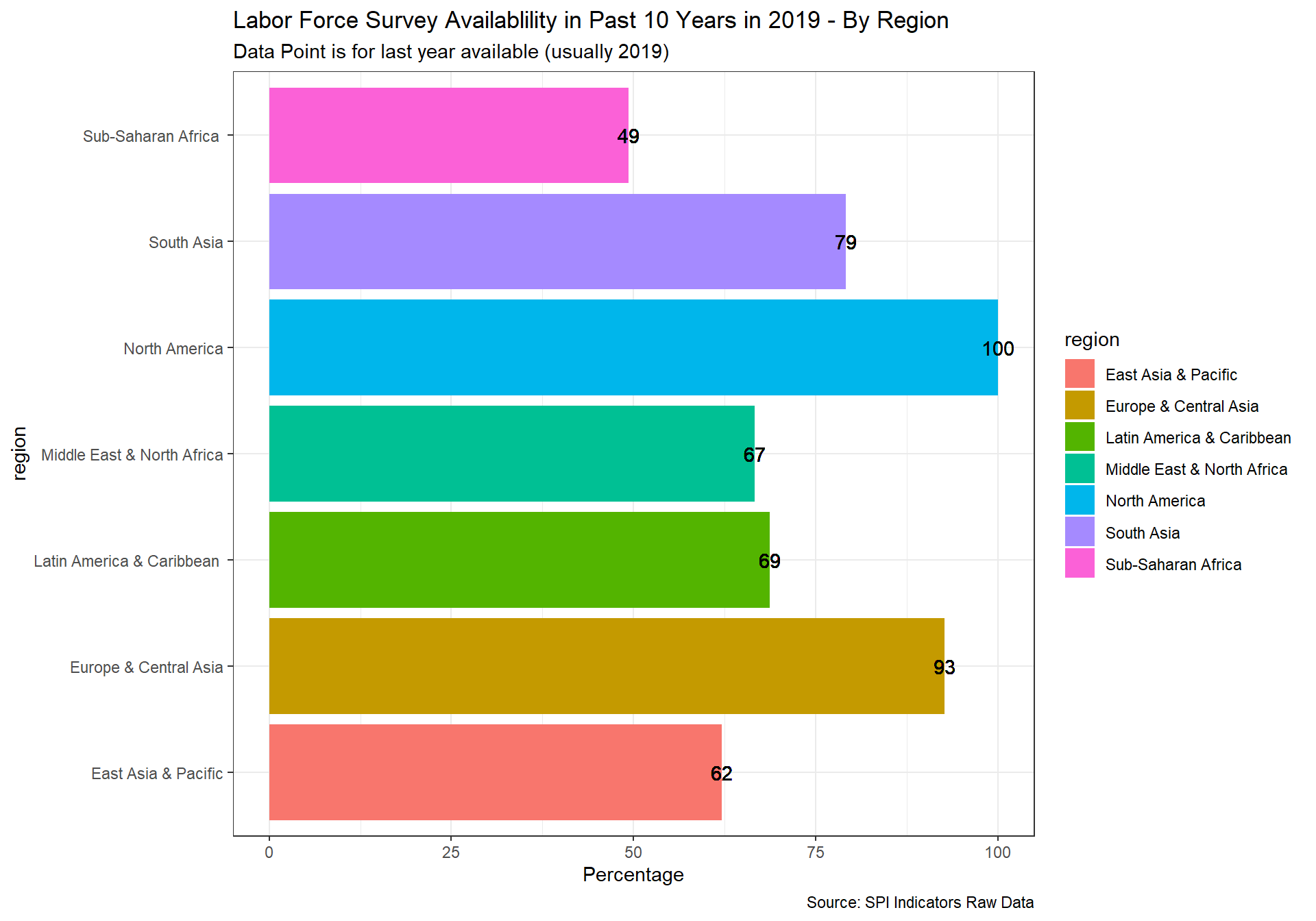
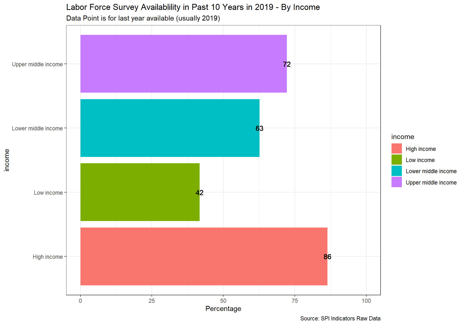
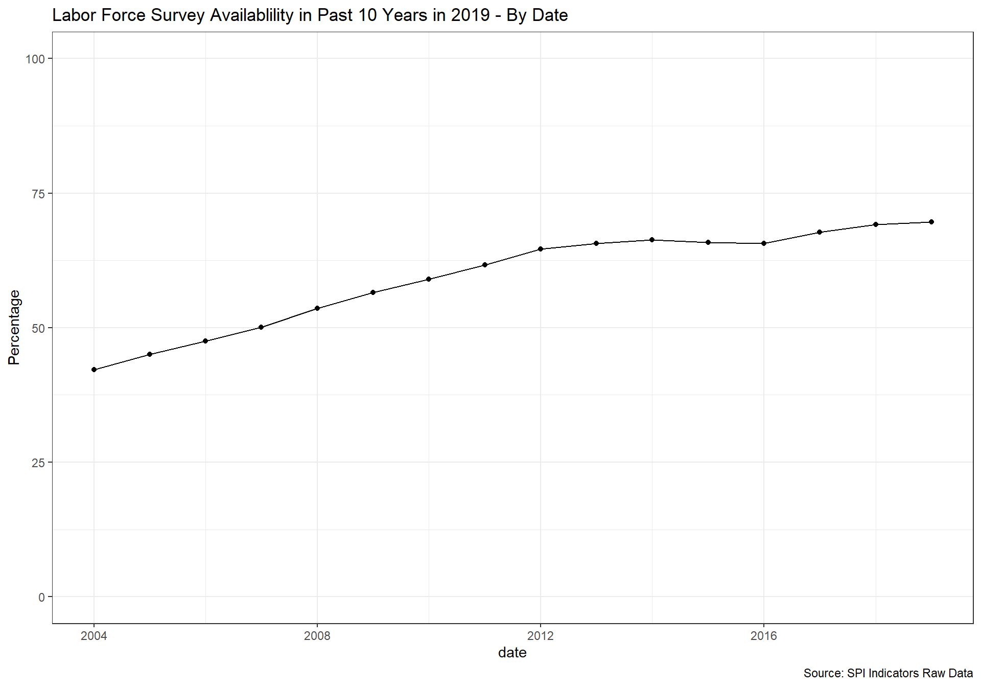
2.4.1.1.6 Labor Force Survey
Labor force survey is a standard household-based survey of work-related statistics at the national and sub-national employment or unemployment levels, rates or trends. The surveys also provide the characteristics of the employed or unemployed, including labor force status by age or gender, breakdowns between employees and the self-employed, public versus private sector employment, multiple job-holding, hiring, job creation, and duration of unemployment.
1 Point. 3 or more surveys done within past 10 years
0.67 Points. 2 surveys done within past 10 years;
0.33 Points. 1 survey done within past 10 years;
0 Points. None within past 10 years
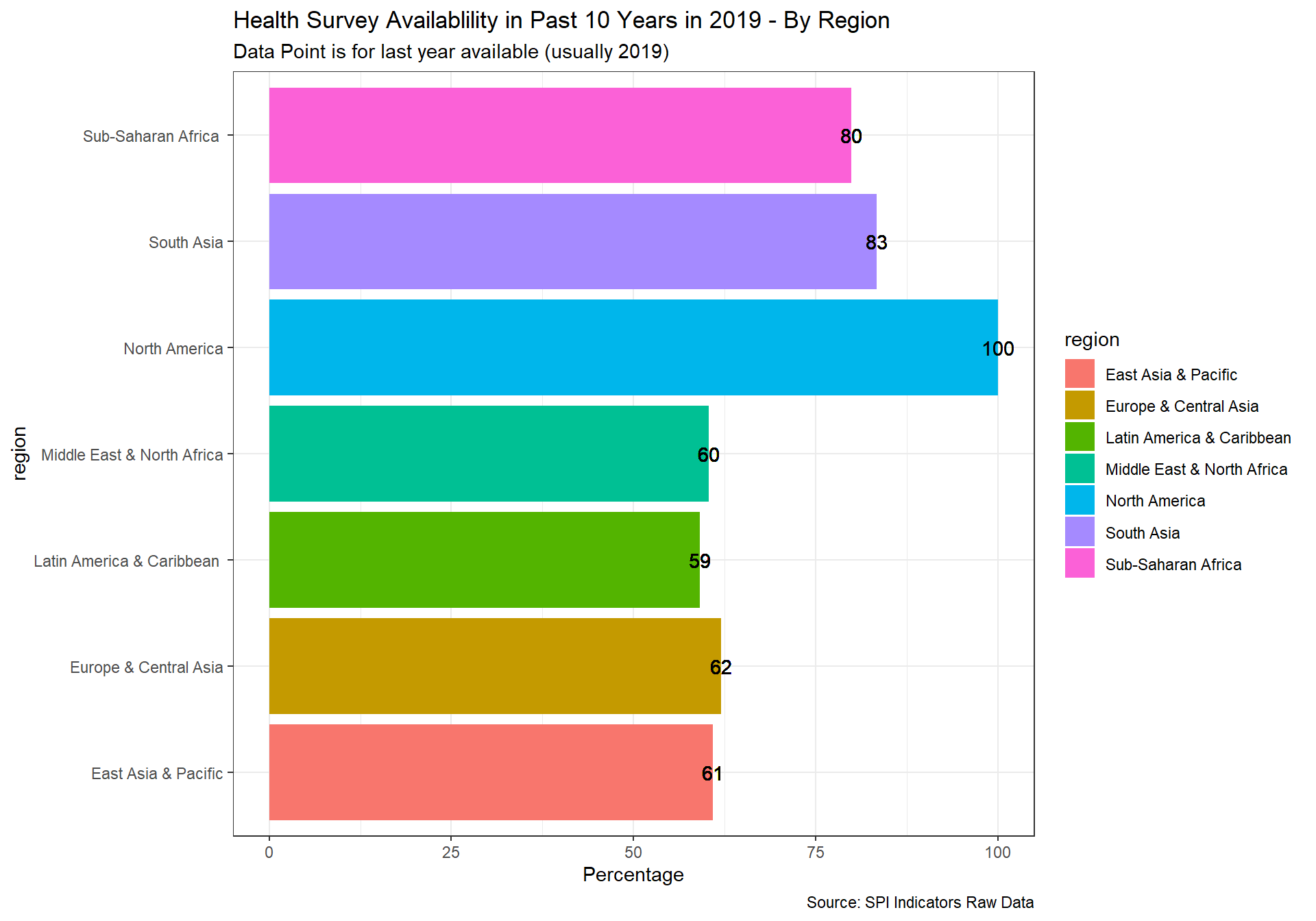
2.4.1.1.7 Health/Demographic survey
Health surveys collect information on various aspects of health of populations, such as health expenditure, access, utilization, and outcomes. They typically include Demographic and Health Surveys. It is recommended that health surveys be conducted at least every 3 to 5 years.
1 Point. 3 or more surveys done within past 10 years
0.67 Points. 2 surveys done within past 10 years;
0.33 Points. 1 survey done within past 10 years;
0 Points. None within past 10 years
2.4.1.1.8 Business/establishment survey
The business/establishment survey provides information on employment, hours, and earnings of employees from a sample of business establishments including private and public, entities that are classified based on an establishment’s principal activity from the business or establishment census. Establishment surveys include surveys of businesses, farms, and institutions. They may ask for information about the establishment itself and/or employee characteristics and demographics.
1 Point. 3 or more surveys done within past 10 years
0.67 Points. 2 surveys done within past 10 years;
0.33 Points. 1 survey done within past 10 years;
0 Points. None within past 10 years
#pull data for population and agriculture census from WDI metadata

df <- WDI_metadata

## Manipulate and clean final data
df <- df %>%
  filter(!is.na(Income.Group))  #keep just countries (drop aggregations)


pop_census_df <- df %>%
  mutate(iso3c=if_else(is.na(Country.Code), Code, Country.Code),
         country=Table.Name) %>%
  select(c('iso3c', 'country', 'date',  'Latest.population.census')  ) %>%
  mutate(last_val=str_extract(Latest.population.census, "\\d{4}") )%>%
    mutate(last_val=as.numeric(last_val)) %>%
    mutate(indicator=case_when(
      (date-last_val<=10) & (date-last_val>=0) ~ 1,
      (date-last_val<=20) & (date-last_val>=0) ~ 0.5,
      TRUE ~ 0 )
    )  %>%
    ungroup() %>%
    select(c('iso3c', 'country', 'date', 'Latest.population.census', 'indicator')  ) %>%
    arrange(date, country)

ag_census_df <- df %>%
  mutate(iso3c=if_else(is.na(Country.Code), Code, Country.Code),
         country=Table.Name) %>%
  select(c('iso3c',  'date',  'Latest.agricultural.census')  ) %>%
  mutate(last_val=str_extract(Latest.agricultural.census, "\\d{4}") )%>%
    mutate(last_val=as.numeric(last_val)) %>%
    mutate(indicator=case_when(
      (date-last_val<=10) & (date-last_val>=0) ~ 1,
      (date-last_val<=20) & (date-last_val>=0) ~ 0.5,
      TRUE ~ 0 )
    )  %>%
    ungroup() %>%
    select(c('iso3c',  'date', 'Latest.agricultural.census', 'indicator')  ) %>%
    arrange(date, iso3c)
census_fun <- function(data, input_var) {
data <- data
input_var <- input_var
#read in csv file.
cs_df <- read_csv(file = paste(raw_dir, '/4.1_SOCS/raw/', data, "_145.csv", sep="" )) %>% #bring in data collected for an original set of 145 countries, then an additional 10, then several more high income counries.
bind_rows(read_csv(file = paste(raw_dir, '/4.1_SOCS/raw/', data, "_10.csv", sep="" ))) %>%
bind_rows(read_csv(file = paste(raw_dir, '/4.1_SOCS/raw/', data, "_high.csv", sep="" ))) %>%
write_excel_csv(path = paste(raw_dir, '/4.1_SOCS/', data, "_manual.csv", sep="" )) %>%
distinct() %>%
group_by(iso3c, country) %>%
rename(input_var = !! input_var) %>%
nest() %>% ## The next chunk of code will split our string with the years of the census (i.e. "2000, 2010") in to separate rows. We will then aggregate up.
mutate(
temp_col = map(
data,
~ str_extract_all(.x$input_var, "\\d{4}") %>%
flatten() %>%
map_chr(~return(.x)) %>%
as_tibble()
)
) %>%
unnest(keep_empty = TRUE) %>% ## Now we have a database with the observations equal to Country*Census observations. From here we can calculate latest census, etc.
mutate(indicator_date=as.numeric(value)) %>%
select('country','indicator_date','input_var')
#append nada data on surveys
cs_df <- cs_df %>%
bind_rows(read_csv(file = paste(raw_dir, '/4.1_SOCS/', data, "_NADA.csv", sep="" ))) %>%
group_by(country, indicator_date) %>%
summarise(input_var=first(na.omit(input_var) ),
nada_dates=first(na.omit(nada_dates) )
) %>%
mutate(indicator_date=if_else(is.na(indicator_date),-99,indicator_date))
#Now calculate our SPI score for this indicator
for (i in 2004:2019) {
temp <- cs_df %>%
mutate(date=i) %>%
mutate(recency_indicator=((date>=indicator_date)) ) %>% #restrict to censuses that do not occur after reference date
mutate(indicator_date=if_else(recency_indicator==TRUE, indicator_date, as.numeric(NA))) %>%
group_by(country, date) %>%
summarise(last_val=max(indicator_date, na.rm=T),
input_var=paste(unique(indicator_date), collapse=","),
nada_dates=first(nada_dates)) %>%
mutate(indicator=case_when(
(date-last_val<=10) & (date-last_val>0) ~ 1,
(date-last_val<=20) & (date-last_val>0) ~ 0.5,
TRUE ~ 0 )
) %>%
ungroup() %>%
select(c( 'country', 'date', 'input_var','nada_dates', 'indicator') ) %>%
arrange(date, country)
assign(paste('temp',i,sep="_"), temp)
}
temp <- temp_2019
for (i in 2004:2018) {
temp <- bind_rows(temp, get(paste('temp',i,sep="_")))
}
temp
}
survey_fun <- function(data, input_var) {
data <- data
input_var <- input_var
#read in csv file that was manually collected.
cs_df <- read_csv(file = paste(raw_dir, '/4.1_SOCS/raw/', data, "_145.csv", sep="" )) %>% #bring in data collected for an original set of 145 countries, then an additional 10, then several more high income counries.
bind_rows(read_csv(file = paste(raw_dir, '/4.1_SOCS/raw/', data, "_10.csv", sep="" ))) %>%
bind_rows(read_csv(file = paste(raw_dir, '/4.1_SOCS/raw/', data, "_high.csv", sep="" ))) %>%
write_excel_csv(path = paste(raw_dir, '/4.1_SOCS/', data, "_manual.csv", sep="" )) %>%
distinct() %>%
group_by( country) %>%
rename(input_var = !! input_var) %>%
nest() %>% ## The next chunk of code will split our string with the years of the census (i.e. "2000, 2010") in to separate rows. We will then aggregate up.
mutate(
temp_col = map(
data,
~ str_extract_all(.x$input_var, "\\d{4}") %>%
flatten() %>%
map_chr(~return(.x)) %>%
as_tibble()
)
) %>%
unnest(keep_empty = TRUE) %>% ## Now we have a database with the observations equal to Country*Census observations. From here we can calculate latest census, etc.
mutate(indicator_date=as.numeric(value)) %>%
select('country','indicator_date','input_var')
#append nada data on surveys
cs_df <- cs_df %>%
bind_rows(read_csv(file = paste(raw_dir, '/4.1_SOCS/', data, "_NADA.csv", sep="" ),
col_types = list(col_character(),col_double(), col_character()))) %>%
group_by(country, indicator_date) %>%
summarise(input_var=first(na.omit(input_var) ),
nada_dates=first(na.omit(nada_dates) )
) %>%
mutate(indicator_date=if_else(is.na(indicator_date),-99,indicator_date))
#Now calculate our SPI score for this indicator
for (i in 2004:2019) {
temp <- cs_df %>%
mutate(date=i) %>%
mutate(window=case_when( #extend the window for more recent years. For instance, 2019 surveys are reported with a lag, so give them two year grace period
date==2019 ~ 12,
date==2018 ~ 11,
TRUE ~ 10
)) %>%
mutate(recency_indicator=((date-indicator_date<=window) & (date-indicator_date>=0)) ) %>% #restrict to surveys inside 10 year period
group_by( country, date) %>% #group by country and create indicator for how many surveys over 10 year period
summarise(indicator=case_when(
sum(recency_indicator)>=3 ~ 1,
sum(recency_indicator)==2 ~ 0.67,
sum(recency_indicator)==1 ~ 0.33,
TRUE ~ 0 ),
input_var=paste(unique(indicator_date), collapse=", "),
nada_dates=first(nada_dates)) %>%
ungroup() %>%
select(c( 'country', 'date', 'input_var','nada_dates', 'indicator') ) %>%
arrange(date, country)
assign(paste('temp',i,sep="_"), temp)
}
temp <- temp_2019
for (i in 2004:2018) {
temp <- bind_rows(temp, get(paste('temp',i,sep="_")))
}
temp
}
#Population Censuses
cs1_df <-pop_census_df %>%
rename(RAW.D4.1.1.POPU=Latest.population.census,
SPI.D4.1.1.POPU=indicator) %>%
select(iso3c, date, starts_with("SPI"), starts_with("RAW"))
#Agriculture census
cs2_df <-ag_census_df %>%
rename(RAW.D4.1.2.AGRI=Latest.agricultural.census,
SPI.D4.1.2.AGRI=indicator) %>%
select(iso3c, date, starts_with("SPI"), starts_with("RAW"))
#Business/establishment census
cs3_df <-census_fun('D4.1.3.CEN.BIZZ', 'BIZZ.CENSUS') %>%
rename(RAW.D4.1.3.BIZZ=input_var,
RAW.D4.1.3.BIZZ.CENSUS_nada=nada_dates,
SPI.D4.1.3.BIZZ=indicator) %>%
select(country, date, starts_with("SPI"), starts_with("RAW"))
#Household Survey on income/ consumption/ expenditure/ budget/ Integrated Survey
cs4_df <-survey_fun('D4.1.4.SVY.HOUS', 'HOUS.SURVEYS') %>%
rename(RAW.D4.1.4.HOUS=input_var,
RAW.D4.1.4.HOUS.SURVEYS_nada=nada_dates,
SPI.D4.1.4.HOUS=indicator) %>%
select(country, date, starts_with("SPI"), starts_with("RAW"))
#Agriculture survey
cs5_df <-survey_fun('D4.1.5.SVY.AGRI', 'AGRI.SURVEYS') %>%
rename(RAW.D4.1.5.AGSVY=input_var,
RAW.D4.1.5.AGRI.SURVEYS_nada=nada_dates,
SPI.D4.1.5.AGSVY=indicator) %>%
select(country, date, starts_with("SPI"), starts_with("RAW"))
#Labor Force Survey
cs6_df <-survey_fun('D4.1.6.SVY.LABR', 'LABR.SURVEYS') %>%
rename(RAW.D4.1.6.LABR=input_var,
RAW.D4.1.6.LABR.SURVEYS_nada=nada_dates,
SPI.D4.1.6.LABR=indicator) %>%
select(country, date, starts_with("SPI"), starts_with("RAW"))
#Health/Demographic survey
cs7_df <-survey_fun('D4.1.7.SVY.HLTH', 'HLTH.SURVEYS') %>%
rename(RAW.D4.1.7.HLTH=input_var,
RAW.D4.1.7.HLTH.SURVEYS_nada=nada_dates,
SPI.D4.1.7.HLTH=indicator) %>%
select(country, date, starts_with("SPI"), starts_with("RAW"))
#Business/establishment survey
cs8_df <-survey_fun('D4.1.8.SVY.BIZZ', 'BIZZ.SURVEYS') %>%
rename(RAW.D4.1.8.BZSVY=input_var,
RAW.D4.1.8.BIZZ.SURVEYS_nada=nada_dates,
SPI.D4.1.8.BZSVY=indicator) %>%
select(country, date, starts_with("SPI"), starts_with("RAW"))
#brind all censuses and surveys together
cs_df <- spi_df_empty %>%
left_join(cs1_df) %>%
left_join(cs2_df) %>%
left_join(cs3_df) %>%
left_join(cs4_df) %>%
left_join(cs5_df) %>%
left_join(cs6_df) %>%
left_join(cs7_df) %>%
left_join(cs8_df)
#add to spi databases
spi_df <- spi_df %>%
left_join(cs_df)
#now do the figures
cs_df_map <- cs_df %>% filter(!is.na(SPI.D4.1.1.POPU))
spi_mapper('cs_df_map', 'SPI.D4.1.1.POPU', 'Population Census Available in Past 20 Years in 2019' )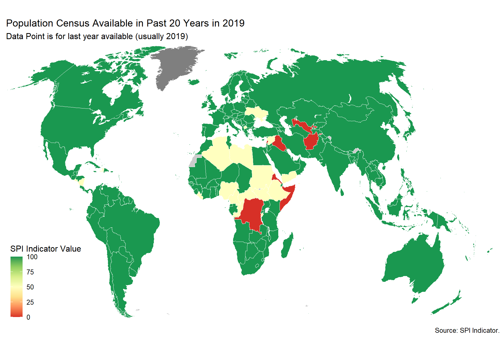
cs_df_map <- cs_df %>%  filter(!is.na(SPI.D4.1.2.AGRI))
spi_mapper('cs_df_map', 'SPI.D4.1.2.AGRI', 'Agriculture Census Available in Past 20 Years in 2019' )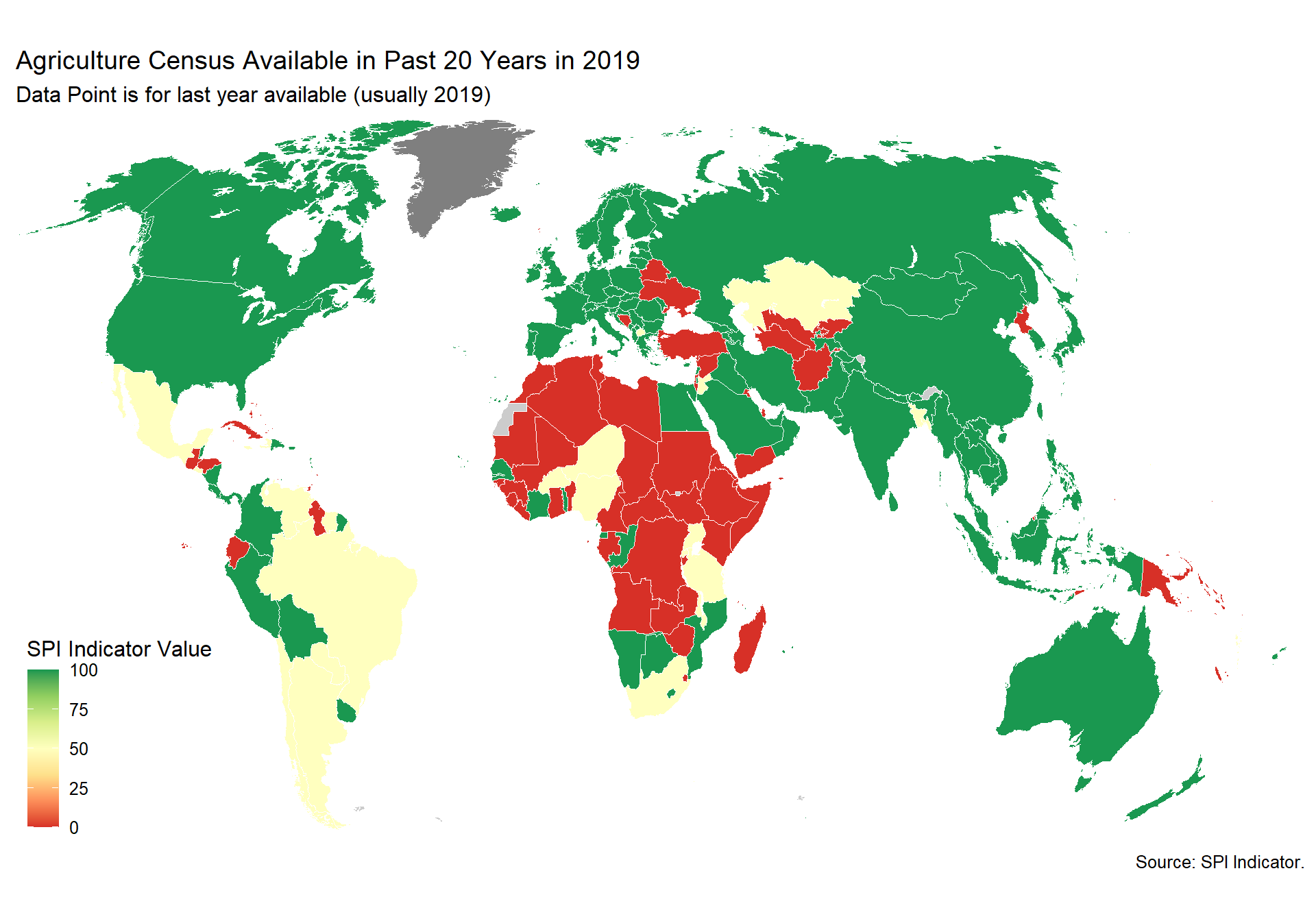
cs_df_map <- cs_df %>%  filter(!is.na(SPI.D4.1.3.BIZZ))
spi_mapper('cs_df_map', 'SPI.D4.1.3.BIZZ', 'Business/Establishment Census Available in Past 20 Years in 2019' )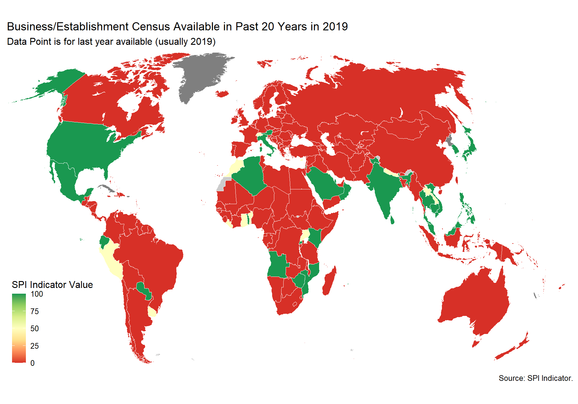
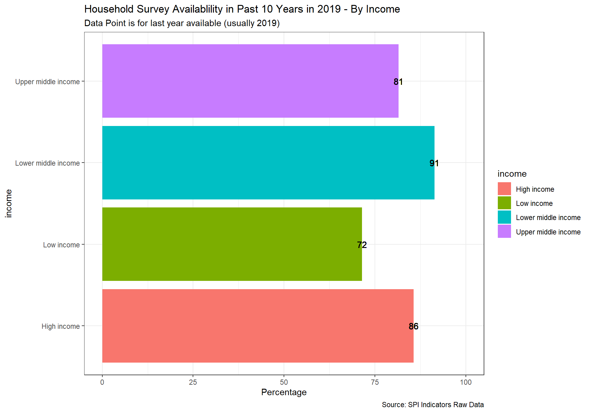
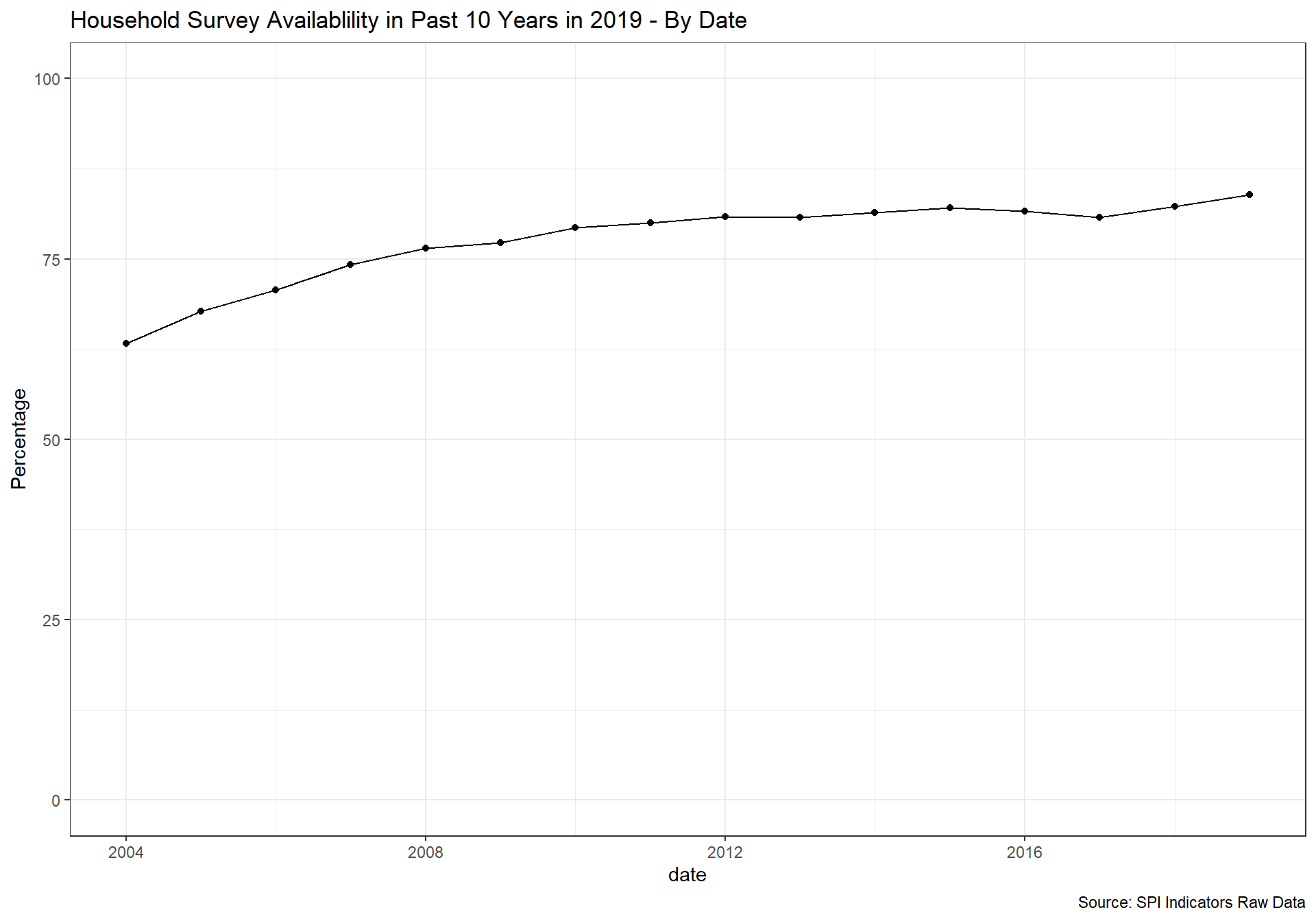
cs_df_map <- cs_df %>%  filter(!is.na(SPI.D4.1.4.HOUS))
spi_mapper('cs_df_map', 'SPI.D4.1.4.HOUS', 'Household Survey Availablility in Past 10 Years in 2019' )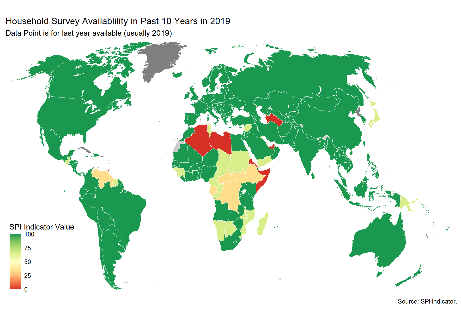
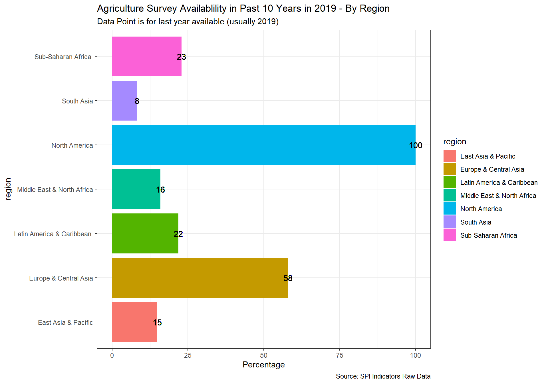
cs_df_map <- cs_df %>%  filter(!is.na(SPI.D4.1.5.AGSVY))
spi_mapper('cs_df_map', 'SPI.D4.1.5.AGSVY', 'Agriculture Survey Availablility in Past 10 Years in 2019' )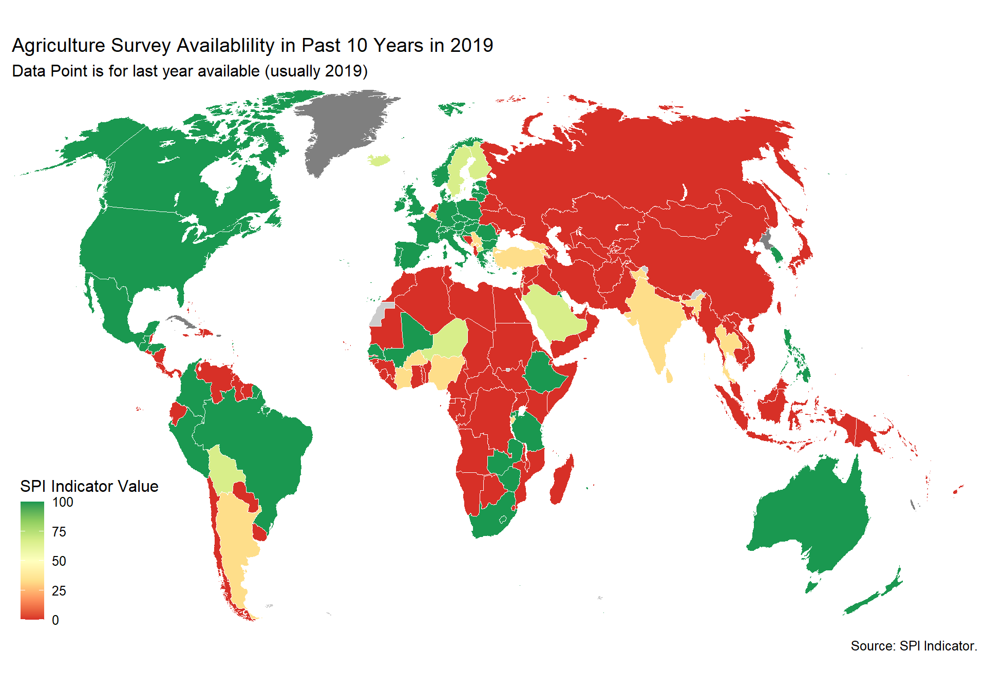
cs_df_map <- cs_df %>%  filter(!is.na(SPI.D4.1.6.LABR))
spi_mapper('cs_df_map', 'SPI.D4.1.6.LABR', 'Labor Force Survey Availablility in Past 10 Years in 2019' )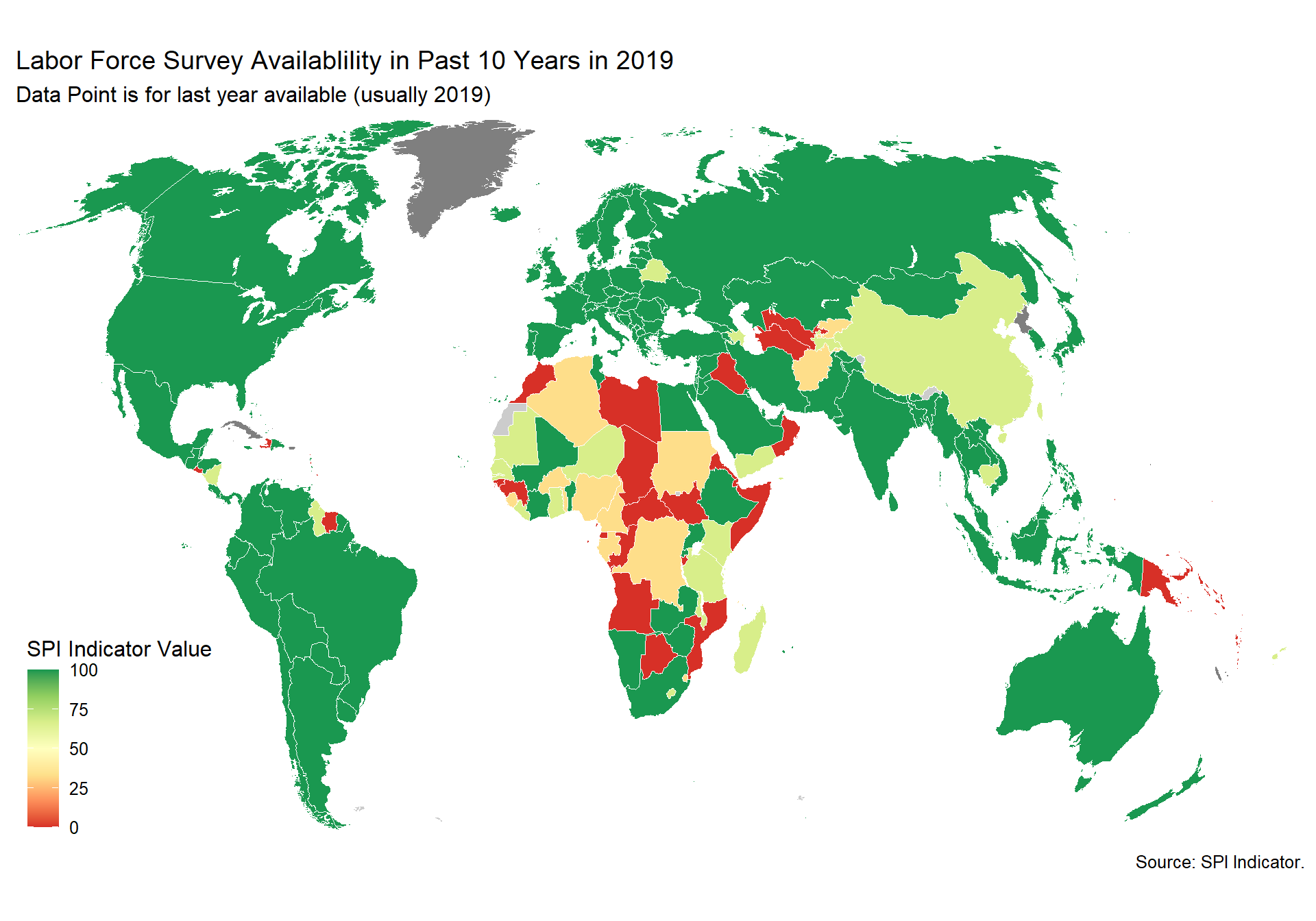
cs_df_map <- cs_df %>% filter(!is.na(SPI.D4.1.7.HLTH))
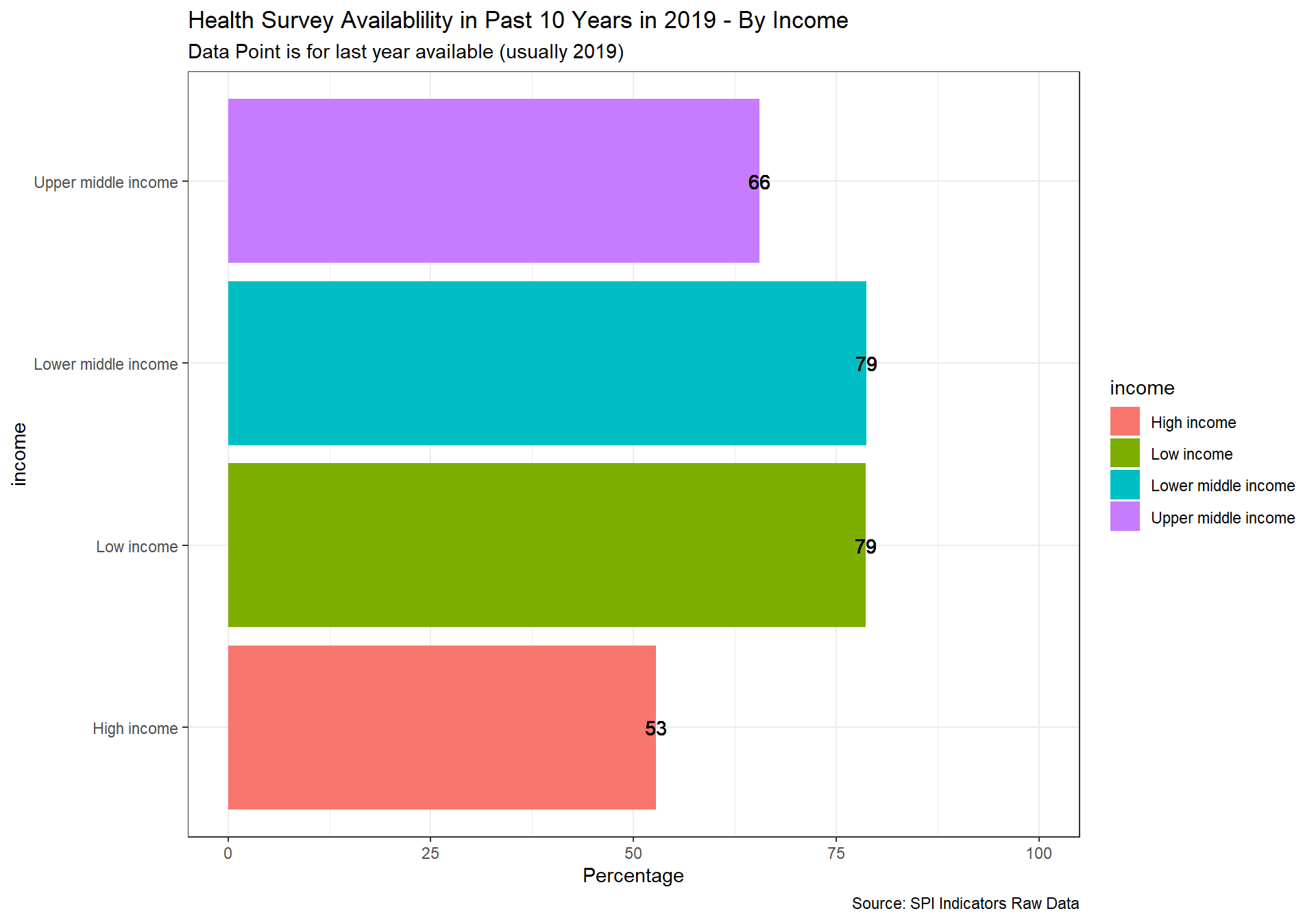
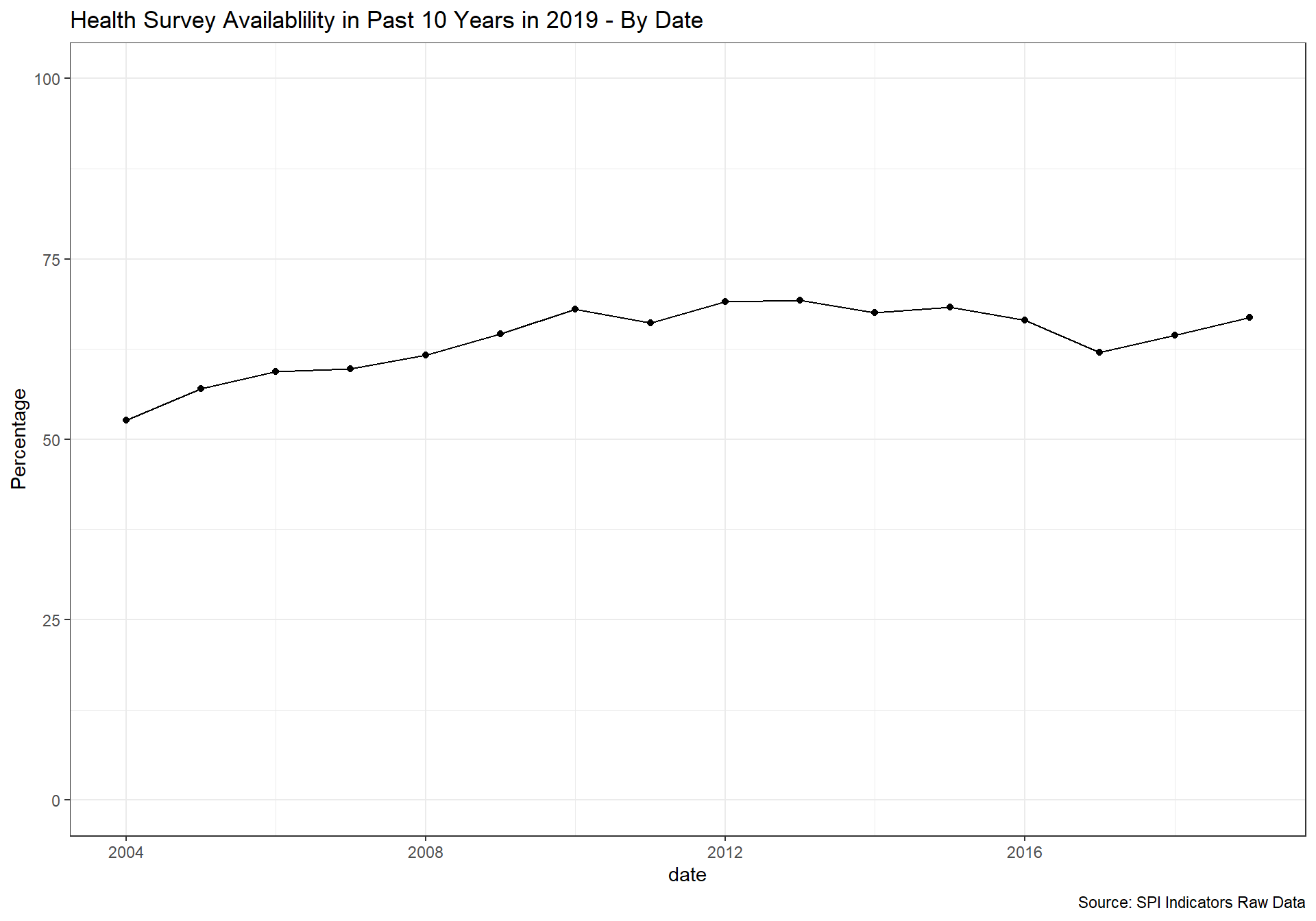
spi_mapper('cs_df_map', 'SPI.D4.1.7.HLTH', 'Health Survey Availablility in Past 10 Years in 2019' )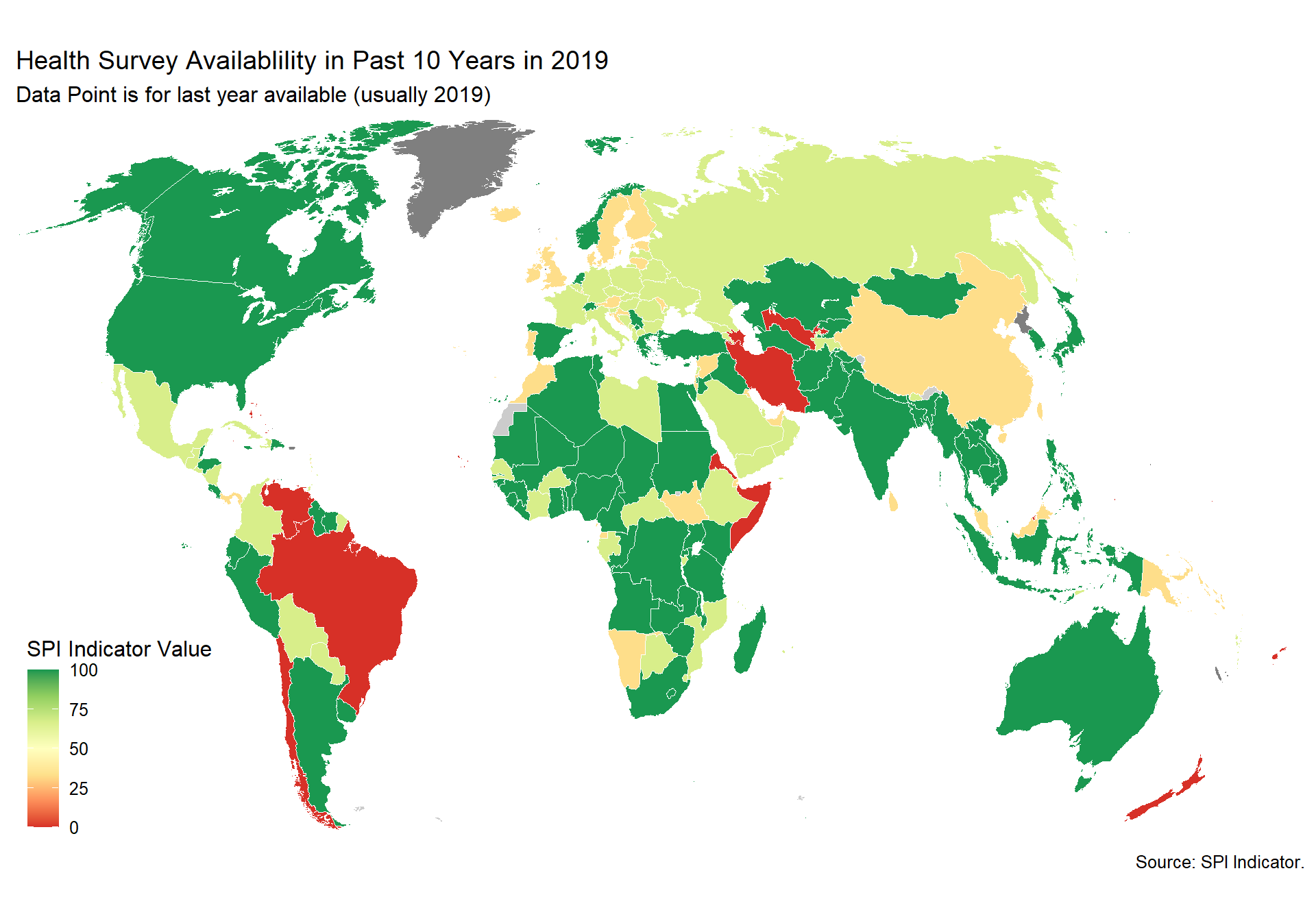
cs_df_map <- cs_df %>% filter(!is.na(SPI.D4.1.8.BZSVY))
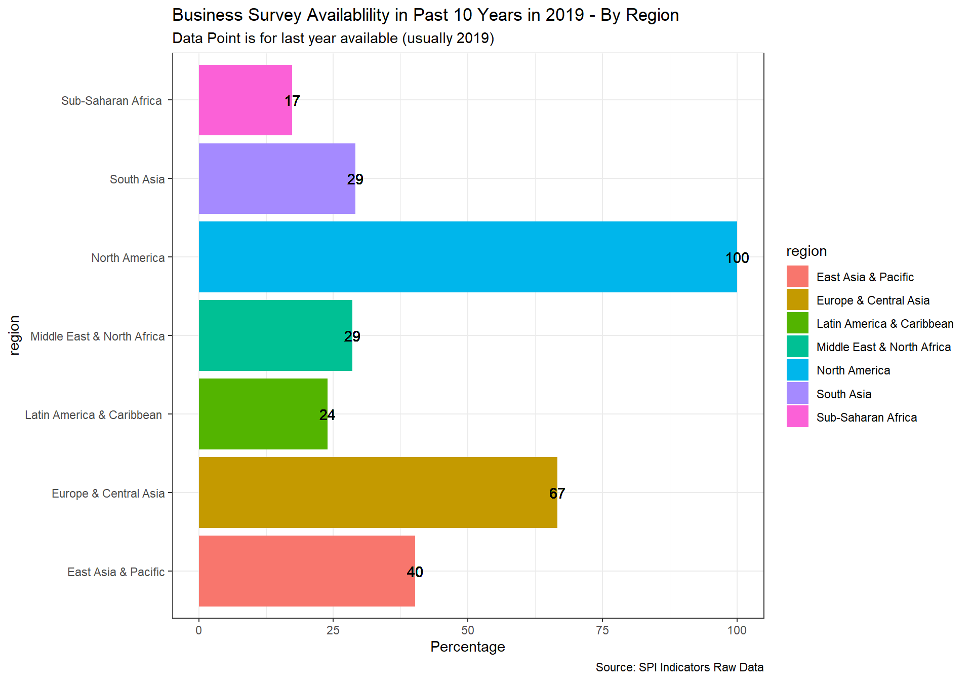
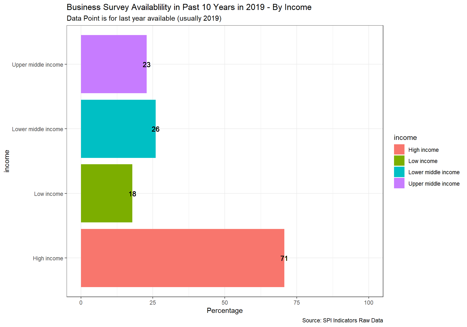
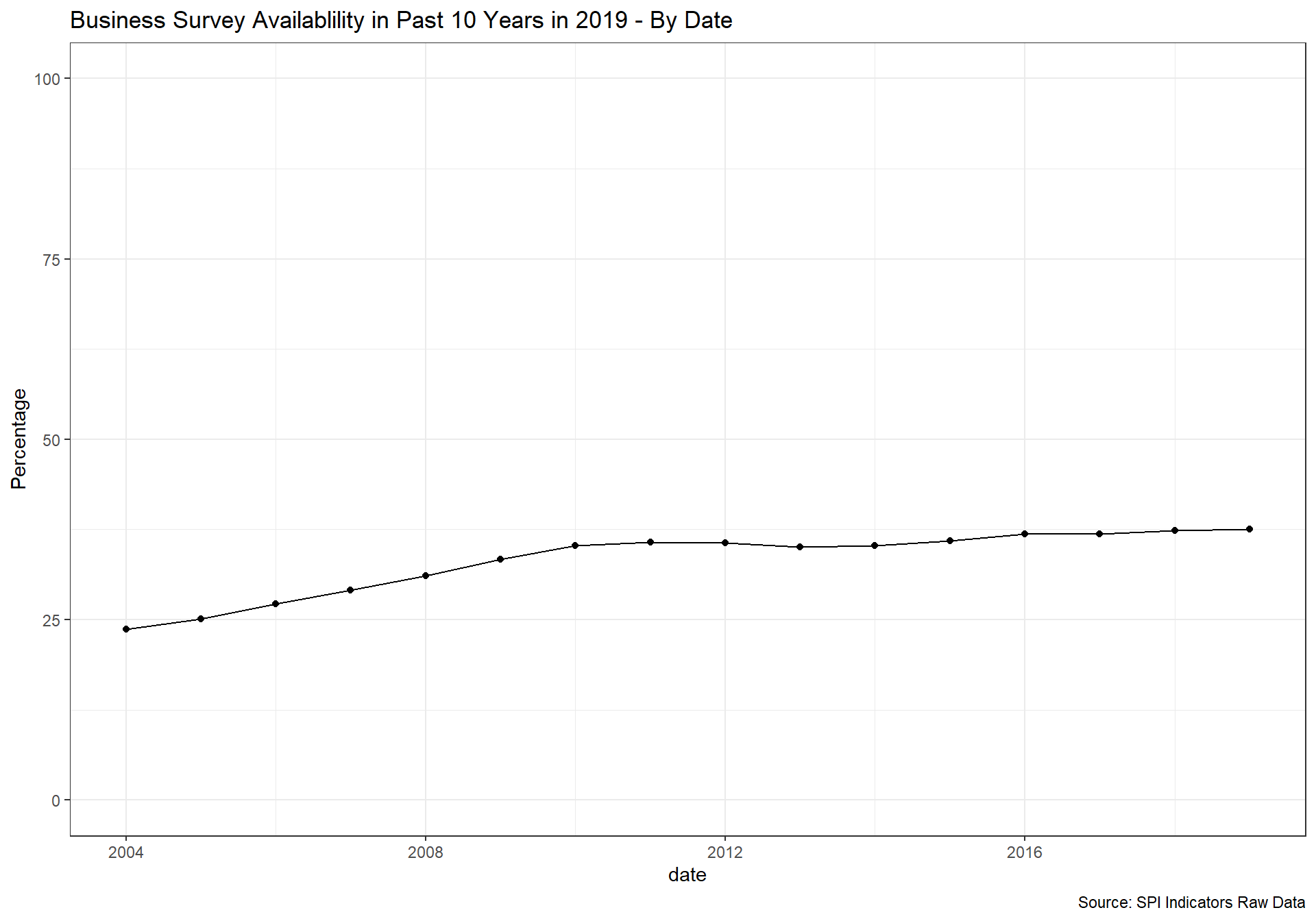
spi_mapper('cs_df_map', 'SPI.D4.1.8.BZSVY', 'Business Survey Availablility in Past 10 Years in 2019' )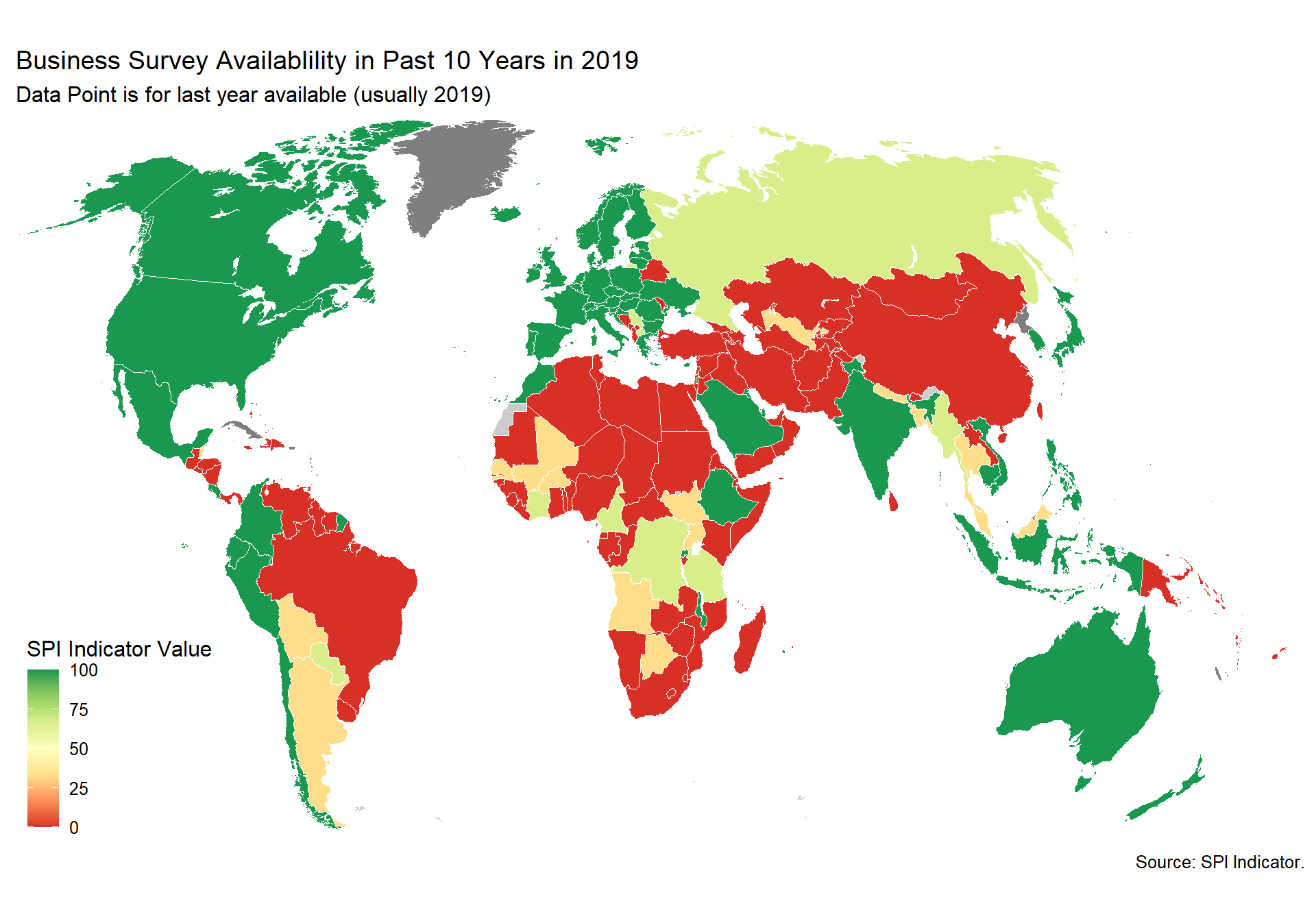
2.4.2 Indicator 4.2: administrative data
The following indicator checks whether administrative data is available for the following topic areas: Social Protection, Education, Population & Health, and Labor
Average score for CRVS indicator. Social Protection, Education, and Labor admin data indicators not included because of lack of established methodology. While our team identified several promising sources for administrative data from the World Bank’s ASPIRE team, UNESCO, and ILO, incomplete coverage across countries made us drop these indicators from our index. A major research and data collection effort is needed from all custodian agencies to fill in this information, so that a more comprehensive picture of administrative data availability can be produced.
–>
–> –>
2.4.2.1 Population & Health Admin Data
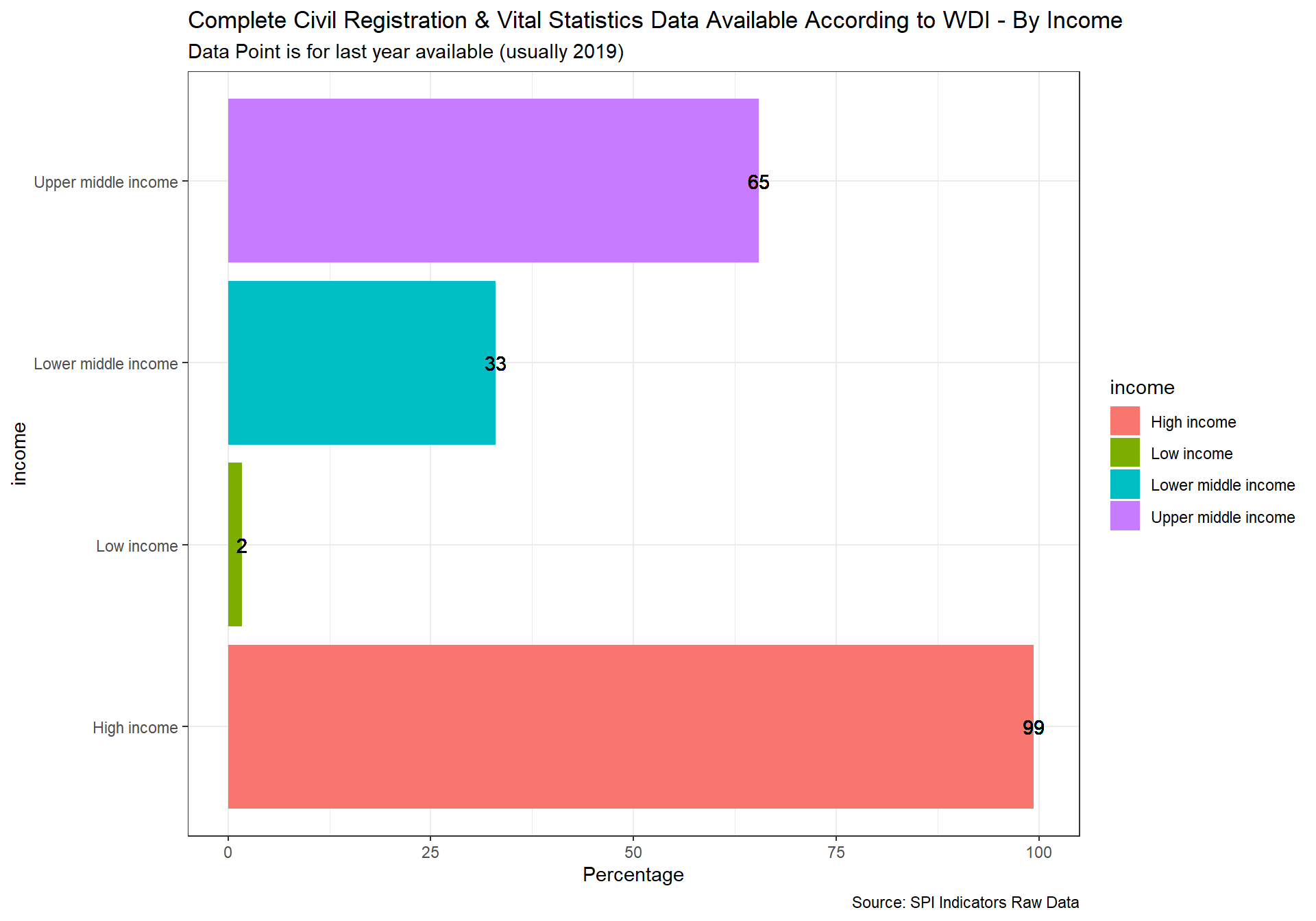
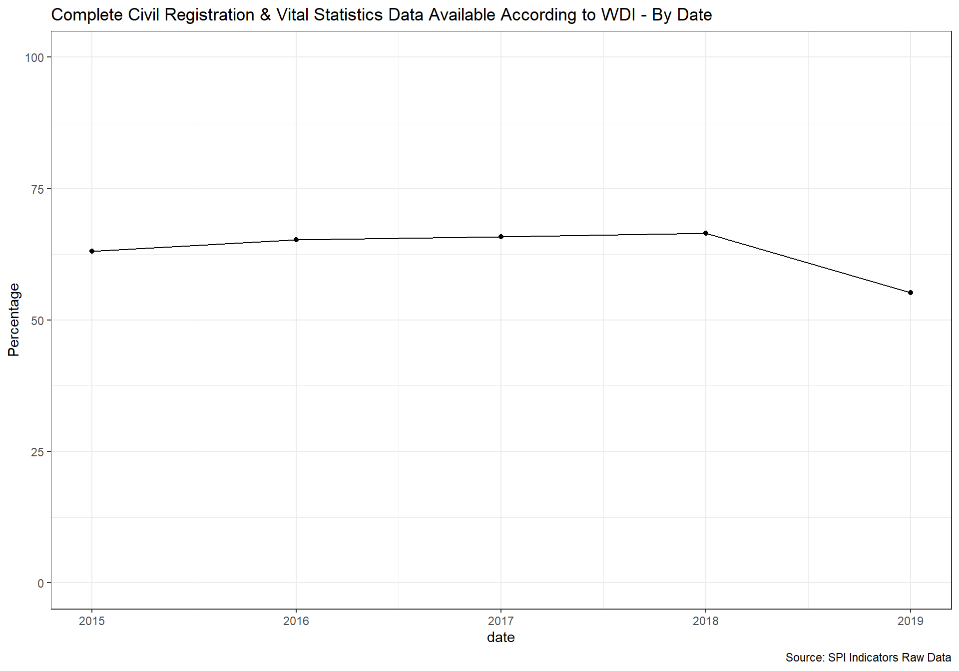
- This indicator is formed using World Bank metadata on whether the Civil Registration and Vital Statistics (CRVS) system is complete in the country.
Civil registration is the act of recording and documenting of vital events in a person’s life (including birth, marriage, divorce, adoption, and death and cause of death) and is a fundamental function of national governments. Birth registration establishes an individual’s legal identity at birth. A legal identity, name, nationality, and proof of age, are important human rights. They enable individuals to be included in various government, social and private services, and include the right to vote, etc. Vital statistics are compiled using civil registration information on these vital events. The availability of reliable and up-to-date vital statistics depends on the level of development of civil registration programs. An effective civil registration and vital statistics (CRVS) system is critical for planning and monitoring programs across several sectors.
Data comes from the UNSD Global SDG monitoring database and also the WDI. Scoring is as follows:
1 Points. Both of at least 90% of births registered and at least 75% of deaths registered
0.5 Points. One of at least 90% of births registered or at least 75% of deaths registered
0 Points. Neither
Source: World Bank WDI Metadata.
#read in data from UNSD database on SDGs
df_birth <- read_csv(file=paste(raw_dir, '4.2_SOAD', 'SG_REG_BRTH90N.csv', sep="/")) %>% #Countries with birth registration data that are at least 90 percent complete (1 = YES; 0 = NO)
filter(date>=2015 & date<=2019) %>%
left_join(spi_df_empty) %>%
transmute(
iso3c=iso3c,
country=country,
date=date,
RAW.D4.2.3.BRTH90=ind_value,
SPI.D4.2.3.BRTH90=if_else(ind_value==1,0.5,0)
)
df_death <- read_csv(file=paste(raw_dir, '4.2_SOAD', 'SG_REG_DETH75N.csv', sep="/")) %>% #Countries with death registration data that are at least 75 percent complete (1 = YES; 0 = NO)
filter(date>=2015& date<=2019) %>%
left_join(spi_df_empty) %>%
transmute(
iso3c=iso3c,
country=country,
date=date,
RAW.D4.2.3.DETH75=ind_value,
SPI.D4.2.3.DETH75=if_else(ind_value==1,0.5,0)
)
#supplement with wdi data
crvs_wdi <- WDI_metadata %>%
select(Country.Code, date, Vital.registration.complete) %>%
mutate(iso3c=Country.Code,
SPI.D4.2.3.WDI=if_else(grepl('Yes', Vital.registration.complete),1,0),
RAW.D4.2.3.CRVS.WDI=Vital.registration.complete) %>%
select(-Country.Code, -Vital.registration.complete)
crvs_df <- df_birth %>%
left_join(df_death) %>%
left_join(crvs_wdi) %>%
mutate(
SPI.D4.2.3.CRVS=SPI.D4.2.3.DETH75+SPI.D4.2.3.BRTH90,
SPI.D4.2.3.CRVS=if_else(is.na(SPI.D4.2.3.CRVS),SPI.D4.2.3.WDI,SPI.D4.2.3.CRVS)) %>%
select(-SPI.D4.2.3.WDI) %>%
group_by(country) %>%
mutate(across(starts_with("SPI"), na.locf, na.rm=FALSE)) %>% #use carry forward to most recent value
mutate(across(starts_with("SPI"), ~if_else(is.na(.),0,.))) %>%
ungroup() %>%
select(c( 'country', 'date','RAW.D4.2.3.BRTH90', 'RAW.D4.2.3.DETH75', 'RAW.D4.2.3.CRVS.WDI', 'SPI.D4.2.3.CRVS') )
#add to spi databases
spi_df <- spi_df %>%
left_join(crvs_df)
crvs_map <- crvs_df
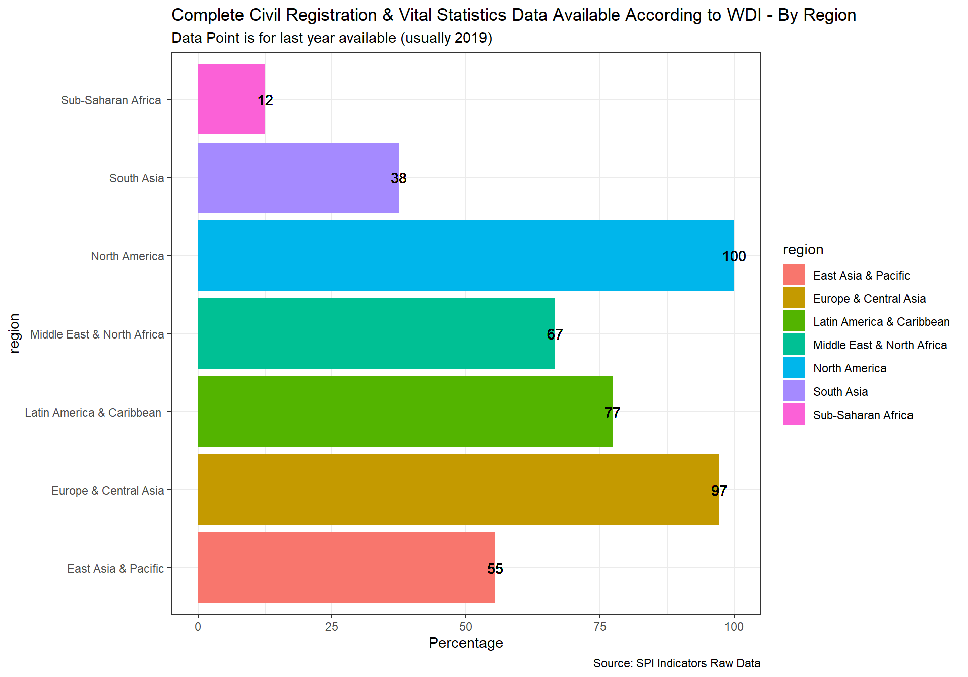
spi_mapper('crvs_map', 'SPI.D4.2.3.CRVS', 'Complete Civil Registration & Vital Statistics Data Available According to WDI' )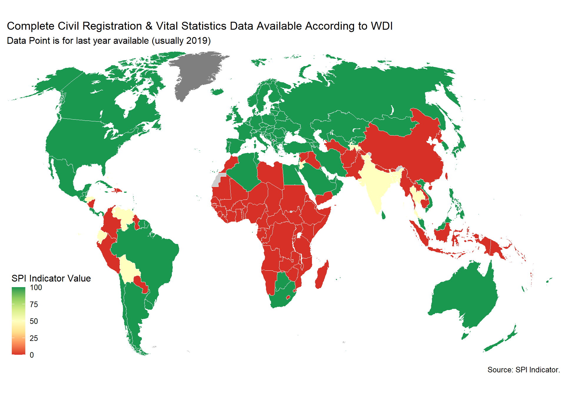
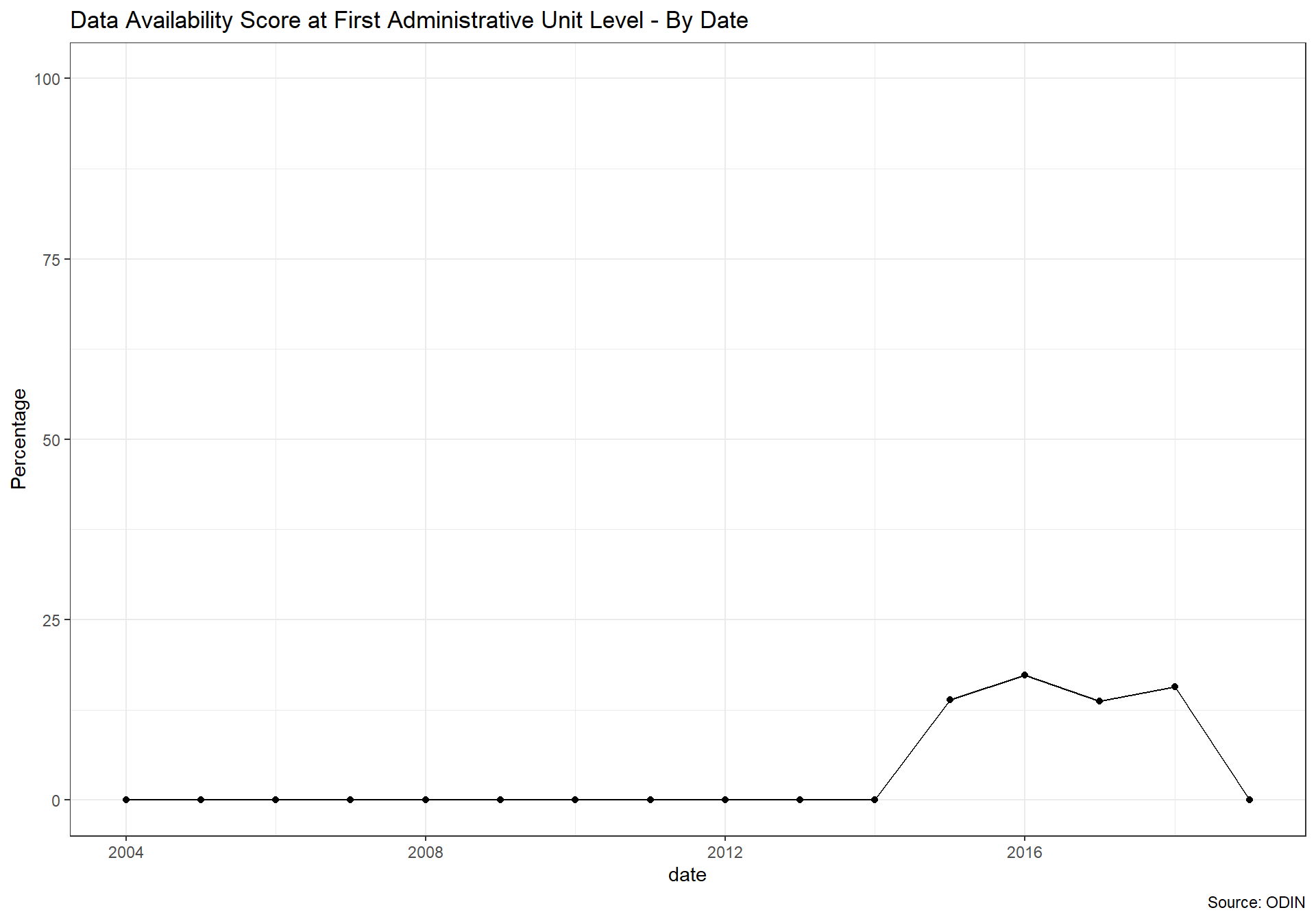
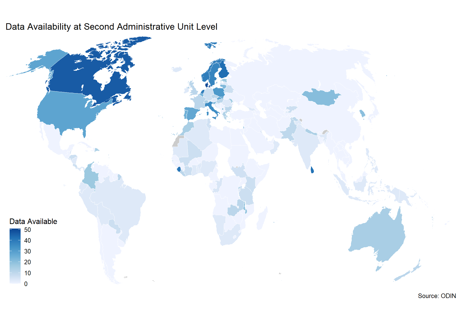
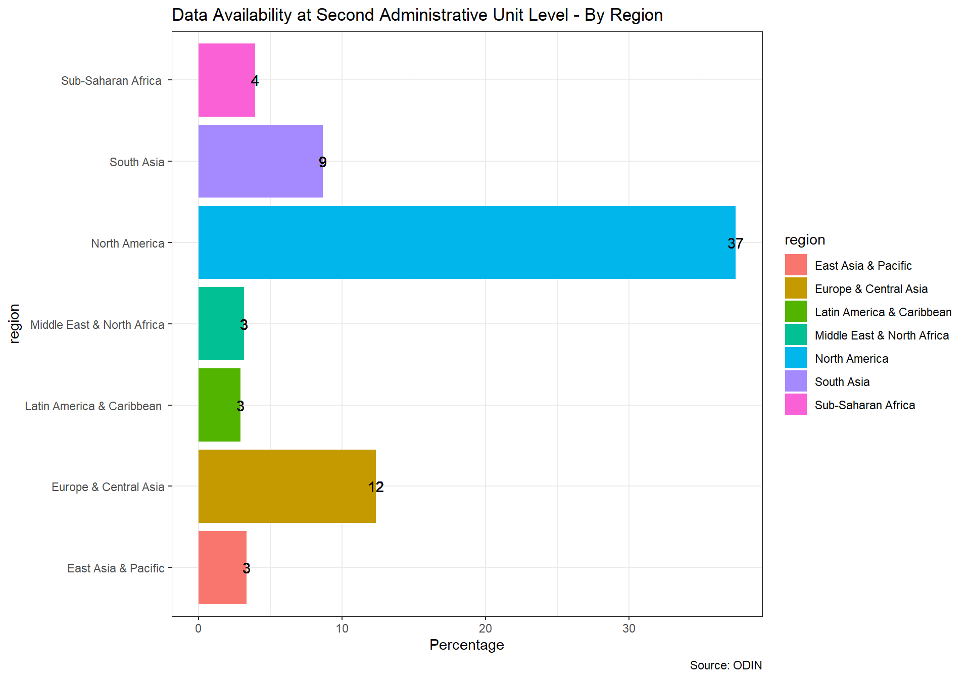
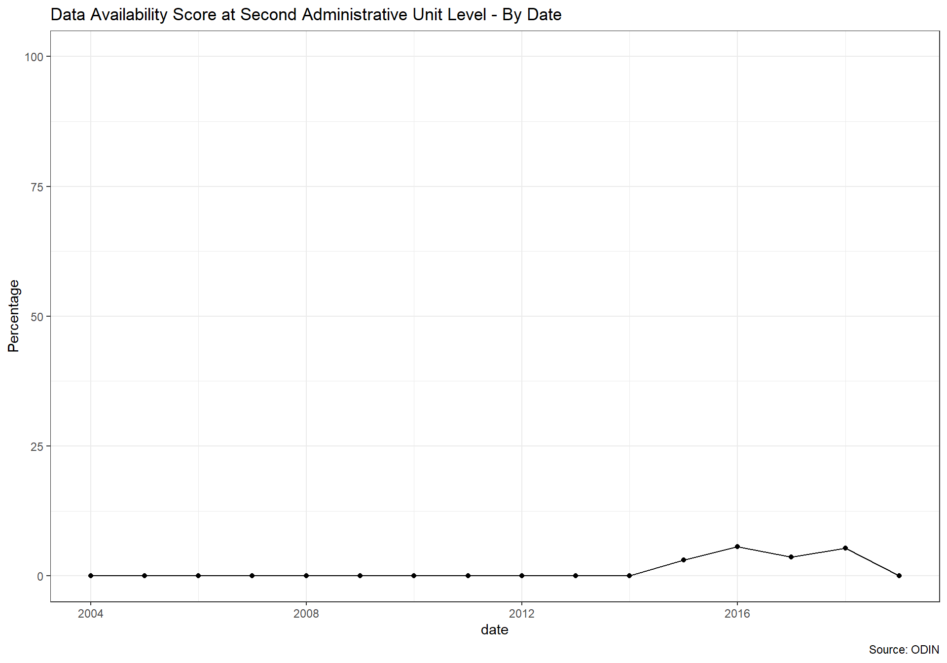
2.4.3 Indicator 4.3: geospatial data
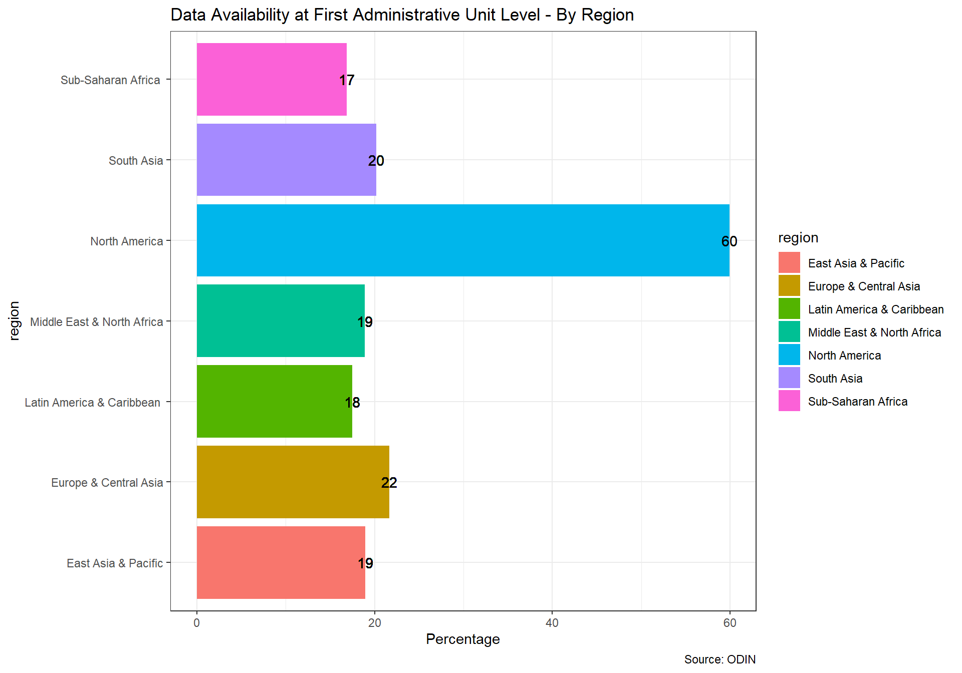
New indicator based on references to geospatial data in metadata relating to content on NSO website. We recognize that this data source provides only limited coverage but consider that it does at least provide some indication of the ability of the national statistical system to produce geospatial data. A major research and data collection effort is needed via GGIM to fill in this information, so that a more comprehensive picture of geospatial data capability at the national level can be produced. Until this is done, it we cannot even assess the scale of the data gaps in a comparable way.
2.4.3.1 Source
Our source for this indicator is Open Data Watch. From Open Data watch:
The Open Data Inventory (ODIN) assesses the coverage and openness of official statistics to help identify gaps, promote open data policies, improve access, and encourage dialogue between national statistical offices (NSOs) and data users. ODIN 2018/19 includes 178 countries, including most all OECD countries. Two-year comparisons are for all countries with two years of data between 2015-2017. Scores can be compared across topics and countries.
We use their indicator on whether indicators are available at the first or second administrative level. To identify the first administrative levels, ODIN largely draws on the ISO 3166-2 standard. In many countries, first administrative levels refer to governorates, regions, or province. No official list exists for the second administrative level classifications. If geographical disaggregation exists that does not qualify as first administrative level, assume that the data are disaggregated to the second administrative level as long as the classification appears to be a further divisions of the first administrative level.
Scoring for the ODIN indicators for geospatial information is below:
- 1 point if all published data in a data category are available at first/second administrative level.
- 0.5 points if some published data in a data category are available at first/second administrative level.
- 0 points if no data are available at this level
There are 21 data categories.
Social Statistics
1. Population and Vital Statistics
2. Education Facilities
3. Education Outcomes
4. Health Facilities
5. Health Outcomes
6. Reproductive Health
7. Gender Statistics
8. Crime and Justice Statistics
9. Poverty Statistics
Economic Statistics
10. National Accounts
11. Labor Statistics
12. Price Indexes
13. Government Finance
14. Money and Banking
15. International Trade
16. Balance of Payments
Environmental Statistics
17. Land Use
18. Resource Use
19. Energy Use
20. Pollution
21. Built Environment
For the first administrative unit: Money & Banking, International Trade, and Balance of Payments are not scored for this element. For various indicators, lenient interpretations are used for first administrative divisions.
For the second administrative unit: Money & Banking, International Trade, Balance of Payments, National Accounts, Government Finance ,Pollution, Energy Use, Price Indexes, and Resource Use are not scored for this element. For various indicators within categories, second administrative level data is not required as well.
In the scores we present below, we show a score between 0 and 1 with a maximum score of 1, which would mean the country has geo data in full for 100% of elements. A score of 0 indicates no data at all for any elements.
More details on the geographic disaggregation considerations can be found in their technical manual:
https://docs.google.com/document/d/1ubPL1l_3im9bjlCVZ6W2ICAy6UAiXl1hGeA1aXImkxI/edit
  #read in ODIN data
  for (i in 2015:2018) {
   temp <- read_csv(paste(raw_dir, '/2.2_DSOA/','ODIN_',i,'.csv', sep=""))  %>%
        as_tibble(.name_repair = 'universal') %>%
        mutate(date=i) %>%
        filter(Data.categories=='All Categories')

    assign(paste('geo_df',i,sep="_"), temp)
  }

#bind different years together
geo_df <- bind_rows(geo_df_2015, geo_df_2016, geo_df_2017, geo_df_2018)


#create geo scores
geo_df <- geo_df %>%
    select(Country.Code, date, First.administrative.level, Second.administrative.level) %>%
    rename(iso3c=Country.Code) %>%
    group_by( iso3c) %>%
    right_join(country_metadata) %>%
    mutate(D4.3.GEO.first.admin.level=if_else(is.na(First.administrative.level), 0, First.administrative.level),
           D4.3.GEO.second.admin.level=if_else(is.na(Second.administrative.level), 0, Second.administrative.level))


#do some quick renaming and formatting
geo_df_temp1 <- geo_df %>%
  rename_with(~paste('RAW',., sep="."), .cols=c('D4.3.GEO.first.admin.level', 'D4.3.GEO.second.admin.level') )


geo_df_temp2 <- geo_df %>%
  mutate(across(c('D4.3.GEO.first.admin.level', 'D4.3.GEO.second.admin.level'), ~./100)) %>%
  rename_with(~paste('SPI',., sep="."), .cols=c('D4.3.GEO.first.admin.level', 'D4.3.GEO.second.admin.level') )

geo_df <- geo_df_temp1 %>%
  left_join(geo_df_temp2)

#add to spi df
spi_df <- spi_df %>%
  left_join(geo_df)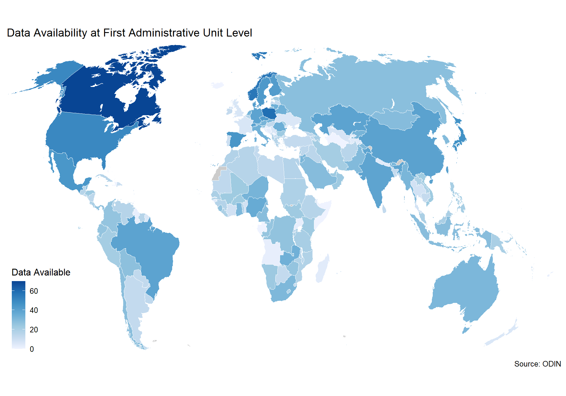
2.4.4 Indicator 4.4: private/citizen generated data
New indicator based on references to private/citizen generated data in metadata relating to content on NSO website. Not included because of lack of established methodology. Currently no comprehensive source exists to measure the use of private and citizen generated data in national statistical systems, and this should be another area where more data collection is needed by the international community.
2.5 Data Infrastructure
Data Infrastructure (5 Indicators):
- 5.1_DILG - Indicator 5.1: legislation and governance
- 5.2_DISM - Indicator 5.2: standards
- 5.3_DISK - Indicator 5.3: skills
- 5.4_DIPN - Indicator 5.4: partnerships
- 5.5_DIFI - Indicator 5.5: finance
2.5.1 Indicator 5.1: legislation and governance
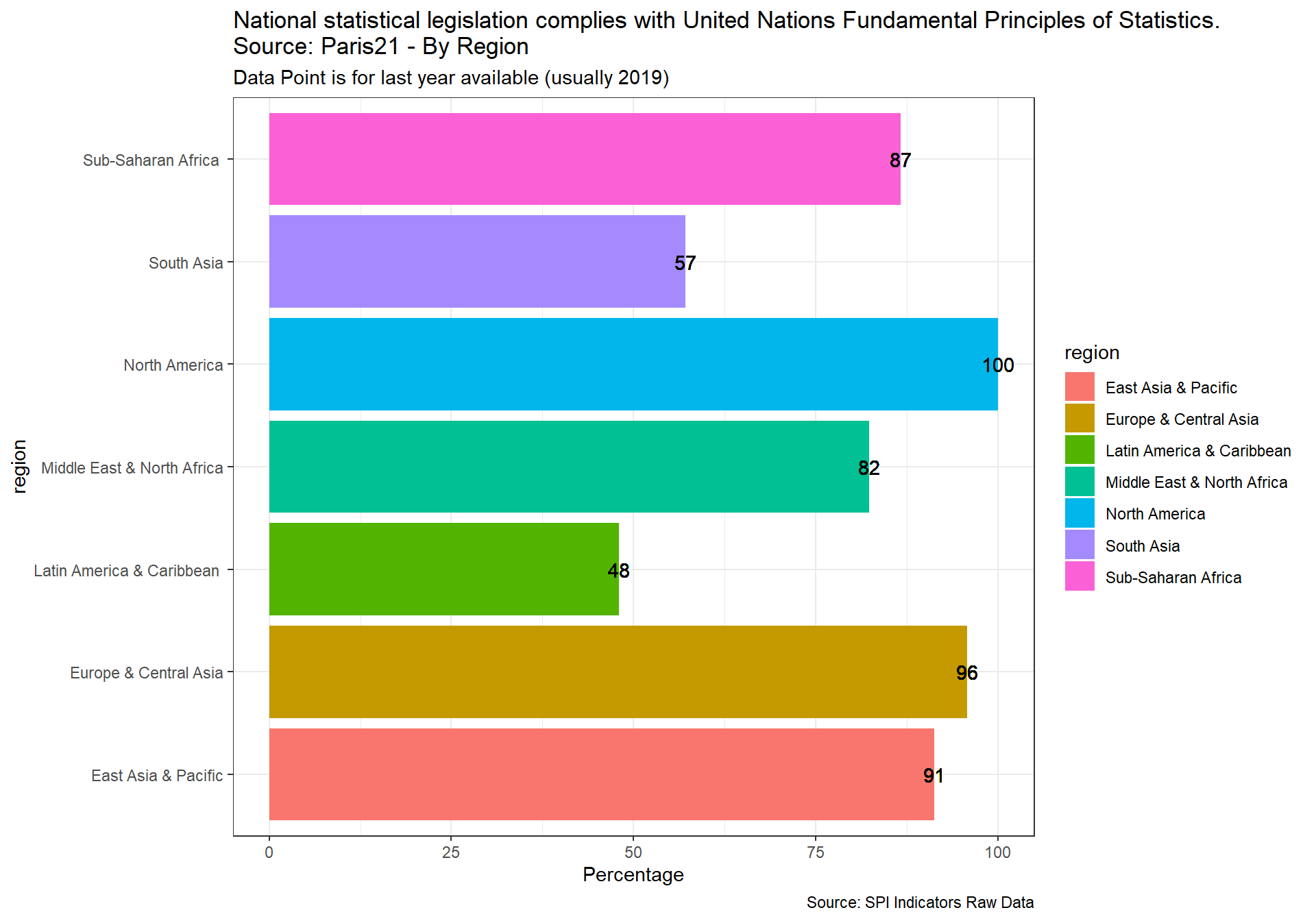
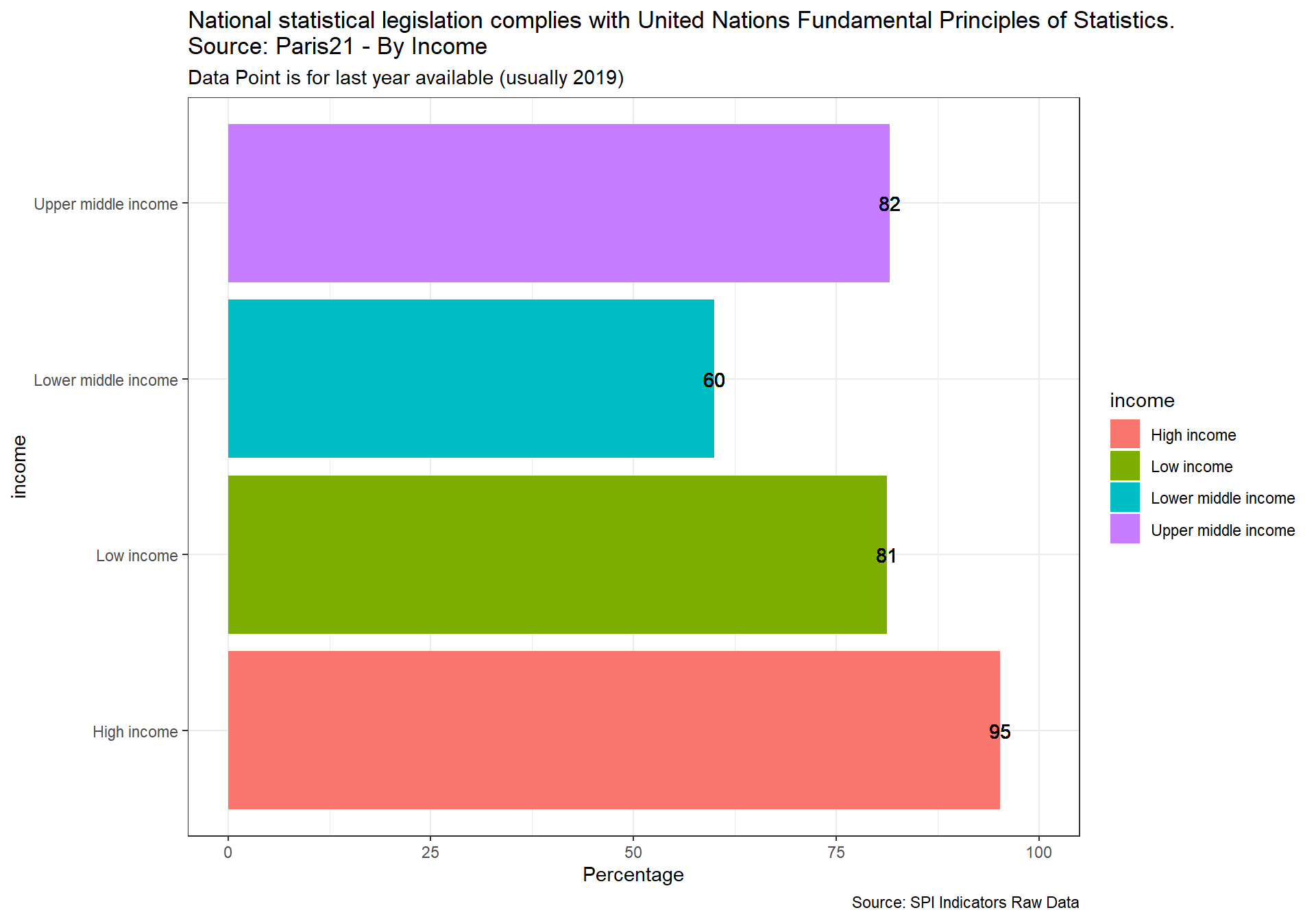
The legislation and governance indicator will be drawn from SDG indicator 17.18.2 (national statistical legislation compliance with UN Fundamental Principles of Official Statistics), existence of National Statistical Council, national statistical strategy generation, national statistical plan. Also include some other legislative aspects that foster good use of statistics eg freedom of information, privacy/transparency, good governance (eg free and fair elections).
This indicator measures whether the national statistical legislation complies with United Nations Fundamental Principles of Statistics (SDG 17.18.2)
Scores is 1 if the country has a national statistical legislation compliant with United Nations Fundamental Principles of Statistics. Scores of 0 given a score of zero.
The source is Paris 21 and UNSD. Data accessed using UNSD SDG API on 2021-03-24
D5.1_DILG <- un_pull('SG_STT_FPOS', '2004', '2019') %>%
  select(iso3c, date,value) %>%
  right_join(spi_df_empty) %>%
  mutate(RAW.D5.1.DILG=if_else((is.na(value) | value=="NaN"),as.numeric(NA), as.numeric(value)),
         SPI.D5.1.DILG=if_else((is.na(value) | value=="NaN"),as.numeric(NA), as.numeric(value))) %>%
  select(-value)
##
## #read in csv file.
## D5.1_DILG2 <- read_csv(file = paste(raw_dir, "5.1_DILG","5.1_DILG.csv", sep="/" )) %>%
##   as_tibble(.name_repair = 'universal') %>%
##   transmute(
##     country=Country,
##     date=Year,
##     SPI.5.1.DILG=Data.Value
##   ) %>%
##     mutate(country=case_when(
##     country=="Bahamas" ~ "Bahamas, The",
##     country=="Bolivia (Plurinational State of)"   ~  "Bolivia"   ,
##     country=="Côte d'Ivoire"  ~  "Cote d'Ivoire"                ,
##     country=="Democratic Republic of the Congo"  ~ "Congo, Dem. Rep."  ,
##     country=="Congo"  ~ "Congo, Rep."        ,
##     country=="Curacao"  ~  "Curacao"       ,
##     country=="Czechia"   ~  "Czech Republic"     ,
##     country=="Egypt"  ~ "Egypt, Arab Rep."        ,
##     country=="Micronesia (Federated States of)"  ~ "Micronesia, Fed. Sts."  ,
##     country=="United Kingdom"   ~  "United Kingdom"    ,
##     country=="Gambia"    ~  "Gambia, The"     ,
##     country=="Iran (Islamic Republic of)"  ~ "Iran, Islamic Rep." ,
##     country=="Kyrgyzstan"   ~  "Kyrgyz Republic"   ,
##     country=="Republic of Korea"   ~ "Korea, Rep."   ,
##     country=="Lao People's Democratic Republic"    ~  "Lao PDR" ,
##     country=="Saint Kitts and Nevis  "   ~ "St. Kitts and Nevis",
##     country=="Saint Lucia"   ~ "St. Lucia",
##     country=="Republic of Moldova"   ~  "Moldova"   ,
##     country=="Democratic People's Republic of Korea"  ~  "Korea, Dem. People’s Rep." ,
##     country=="Slovakia"   ~  "Slovak Republic"             ,
##     country=="United Republic of Tanzania"   ~  "Tanzania" ,
##     country=="United States of America"  ~ "United States"  ,
##     country=="Saint Vincent and the Grenadines" ~ "St. Vincent and the Grenadines" ,
##     country=="Venezuela (Bolivarian Republic of)"  ~  "Venezuela, RB"   ,
##     country=="British Virgin Islands"  ~  "British Virgin Islands" ,
##     country=="Viet Nam"  ~ "Vietnam"        ,
##     country=="Yemen"  ~ "Yemen, Rep.",
##     country=="United Kingdom of Great Britain and Northern Ireland" ~ "United Kingdom",
##     TRUE ~ country
##   )) %>%
##   mutate(RAW.5.1.DILG=if_else(SPI.5.1.DILG=='no data',as.character(NA), SPI.5.1.DILG),
##          SPI.5.1.DILG=if_else(SPI.5.1.DILG=='no data',as.numeric(NA), as.numeric(SPI.5.1.DILG))) %>%
##   right_join(spi_df_empty)

#add to spi databases
spi_df <- spi_df %>%
  left_join(D5.1_DILG)


D5.1_DILG_map <- D5.1_DILG %>%
  filter(!is.na(SPI.D5.1.DILG))

spi_mapper('D5.1_DILG_map', 'RAW.D5.1.DILG', 'National statistical legislation complies with United Nations Fundamental Principles of Statistics. Source: Paris21')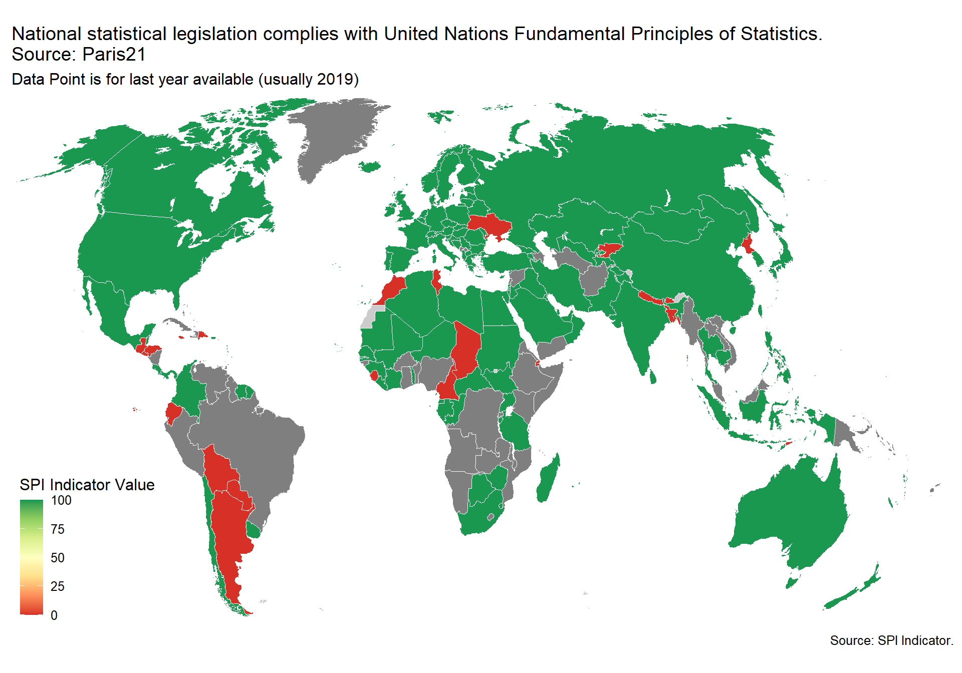
2.5.2 Indicator 5.2: standards
Average score for Standards and Methods indicators. In this release of the SPI the data and methods used for this indicator are the same as for the previous SPI. Further work could improve the validity of this indicator and reduce the risk that countries may be incentivized to adopt only traditional standards and methods and neglect innovative solutions that may be more valid in the current context.
#pull data for several of the standards from WDI metadata

df <- WDI_metadata

## Manipulate and clean final data
df <- df %>%
  filter(!is.na(Income.Group))  #keep just countries (drop aggregations)

#pull IMF country codes for merging
imf_codes <- read_csv(file=paste(raw_dir, "metadata","IMF_country_codes.csv", sep="/" ))
2.5.2.1 5.2.1 System of National Accounts in use
The national accounts data are compiled using the concepts, definitions, framework, and methodology of the System of National Account 2008 (SNA2008) or European System of National and Regional Accounts (ESA 2010). The manual has evolved to meet the changing economic structure, to follow systematic accounting and ensure international compatibility.
Scoring: 1 point for using SNA2008 or ESA 2010, 0.5 points for using SNA 1993 or ESA 1995, 0 points otherwise
#read in metadata file.
D5.2.1.SNAU <- df %>%
  mutate(iso3c=if_else(is.na(Country.Code), Code, Country.Code),
         country=Table.Name) %>%
  select(c('iso3c', 'country', 'date',  'System.of.National.Accounts')  ) %>%
  mutate(SNAU=System.of.National.Accounts) %>%
  mutate(SNAU=str_extract(SNAU, "\\d{4}") ) %>%
  mutate(SPI.D5.2.1.SNAU=case_when(
    SNAU=="2008" ~ 1,
    SNAU=="1993" ~ 0.5,
    TRUE ~ 0
  ),
      RAW.D5.2.1.SNAU=System.of.National.Accounts) %>%
  arrange(date, country) %>%
  select(iso3c,  date,RAW.D5.2.1.SNAU, SPI.D5.2.1.SNAU  )
2.5.2.2 5.2.2 National Accounts base year
National accounts base year is the year used as the base period for constant price calculations in the country’s national accounts. It is recommended that the base year of constant price estimates be changed periodically to reflect changes in economic structure and relative prices.
1 point for chained price, 0.5 for reference period within past 10 years, 0 points otherwise.
D5.2.2.NABY <- df %>%
  mutate(iso3c=if_else(is.na(Country.Code), Code, Country.Code),
         country=Table.Name) %>%
  select(c('iso3c', 'country', 'date',  'National.accounts.base.year')  ) %>%
  mutate(NABY=National.accounts.base.year) %>%
  mutate(NABY_dates=gsub("\\d{2}/","",NABY) ) %>%
  mutate(NABY_dates=str_extract(NABY_dates, "\\d{4}") ) %>%
  mutate(NABY_dates=if_else(NABY=="20015/2016","2016",NABY_dates)) %>% #fix an issue in WDI metadata
  mutate(SPI.D5.2.2.NABY=case_when(
    NABY=="Original chained constant price data are rescaled." ~ 1,
    (date-as.numeric(NABY_dates))<=10 ~ 0.5, #within 10 years of reference period
    TRUE ~ 0
  ),
  RAW.D5.2.2.NABY=NABY)  %>%
  select(iso3c,  date, RAW.D5.2.2.NABY, SPI.D5.2.2.NABY  ) %>%
  arrange(date)
2.5.2.3 5.2.3 Classification of national industry
The industrial production data are compiled using the International Standard Industrial Classification of All Economic Activities (ISIC) Rev.4 and Statistical Classification of Economic Activities in the European Community (NACE) Rev.2. ISIC Rev.4 is a standard classification of economic activities arranged so that entities can be classified per the activity they carry out using criteria such as input, output and use of the products produced, more emphasis has been given to the character of the production process in defining and delineating ISIC classes for international comparability. The manual and classification have changed to cover the complete scope of industrial production, employment, and GDP and other statistical areas.
1 Point. Latest version is adopted (ISIC Rev 4, NACE Rev 2 or a compatible classification)
0.5 Points. Previous version is used (ISIC Rev 3, NACE Rev 1 or a compatible classification)
0 Points. Otherwise
#read in csv file.
D5.2.3.CNIN <- read_csv(file = paste(raw_dir, "5.2_DISM","D5.2.3.CNIN.csv", sep="/" )) %>%
  mutate(SPI.D5.2.3.CNIN=case_when(
    str_to_lower(CNIN)=="nace rev2" | str_to_lower(CNIN)=="rev4" ~ 1,
    str_to_lower(CNIN)=="nace rev1" | str_to_lower(CNIN)=="rev3" ~ 0.5,
    TRUE ~ 0
  ),
  RAW.D5.2.3.CNIN=CNIN)  %>%
  select(iso3c, country, date, RAW.D5.2.3.CNIN, SPI.D5.2.3.CNIN  ) %>%
  arrange(date, country)
2.5.2.4 5.2.4 CPI base year
Consumer Price Index serves as indicators of inflation and reflects changes in the
cost of acquiring a fixed basket of goods and services by the average consumer.
Weights are usually derived from consumer expenditure surveys and the CPI base year
refers to the year the weights were derived. It is recommended that the base year be
changed periodically to reflect changes in expenditure structure.
1 Point. Annual chain linking. 0.5 Points. Base year in last 10 years. 0 points. Otherwise
#read in csv file.
D5.2.4.CPIBY <- read_csv(file = paste(raw_dir, "5.2_DISM","D5.2.4.CPIBY.csv", sep="/" )) %>%
  mutate(SPI.D5.2.4.CPIBY=case_when(
    CPIBY=="annual chained" ~ 1,
    (date-as.numeric(CPIBY))<=10 ~ 0.5, #within 10 years of reference period
    TRUE ~ 0
  ),
  RAW.D5.2.4.CPIBY=CPIBY)  %>%
  select(iso3c, country, date, RAW.D5.2.4.CPIBY, SPI.D5.2.4.CPIBY  ) %>%
  arrange(date, country)

#####
## IMF Data
#####

#use alternative data source provided by the IMF

#read in data on when the weights were last updated to measure if annual chain linking is done
D5.2.4.COICOP.WGT <-   read_excel(path=paste(raw_dir, "5.2_DISM","2020.11.04_Compiled Data for World Bank.xlsx", sep="/" ),
                               sheet = "COICOP Month_Last Change",
                               skip=2
                               ) %>%
  as_tibble(.name_repair='universal') %>%
  rename(
    IMF_code=Code,
    IMF_country=Country_revised
  ) %>%
  mutate(IMF_code=as.numeric(IMF_code)) %>%
  left_join(imf_codes)


#read in last time the CPI reference period is updated to fill in rest of info
D5.2.4.CPI.REF <-  read_excel(path=paste(raw_dir, "5.2_DISM","2020.11.04_Compiled Data for World Bank.xlsx", sep="/" ),
                               sheet = "CPI Reference Period Review"
                               ) %>%
  as_tibble(.name_repair='universal') %>%
  rename(IMF_country=country) %>%
  left_join(D5.2.4.COICOP.WGT) #merge CPI weights

#now calculate whether annual chain linking is used and CPI base year from scratch using this info
D5.2.4.CPIBY.IMF.RAW <- D5.2.4.CPI.REF %>%
  filter(!is.na(iso3c)) %>%
  mutate(CPI_ref_period=str_sub(CPI.reference.period.review,1,4),
         CPI_ref_period=as.numeric(CPI_ref_period),
         CPI_weight_change=str_sub(last_change,1,4),
         CPI_weight_change=as.numeric(CPI_weight_change)) %>%
  mutate(RAW.D5.2.4.CPIBY.IMF=if_else((CPI_weight_change>=2019 & CPI_ref_period<2020), "annual chained",as.character(CPI_ref_period))) %>%
  mutate(RAW.D5.2.4.CPIBY.IMF=if_else((iso3c=='AUS' | iso3c=='NZL'),"annual chained",as.character(RAW.D5.2.4.CPIBY.IMF))) #replace Australia and New Zealand as annual chain linking.  They use quarterly cpi releases and do not show up in this dataset

#score from 2010 to 2019
if (exists('D5.2.4.CPIBY.IMF')) {
    rm(D5.2.4.CPIBY.IMF)
}

for (i in c(2015:2019)) {
  temp <- D5.2.4.CPIBY.IMF.RAW %>%
    mutate(date=i) %>%
    mutate(SPI.D5.2.4.CPIBY.IMF=case_when(
      RAW.D5.2.4.CPIBY.IMF=="annual chained" ~ 1,
      (date-as.numeric(RAW.D5.2.4.CPIBY.IMF))<=10 ~ 0.5, #within 10 years of reference period
      TRUE ~ 0
    )) %>%
    select(iso3c, date, RAW.D5.2.4.CPIBY.IMF, SPI.D5.2.4.CPIBY.IMF  ) %>%
    arrange(date, iso3c)

  if (!exists('D5.2.4.CPIBY.IMF')) {
    D5.2.4.CPIBY.IMF <- temp
  } else {
    D5.2.4.CPIBY.IMF <- D5.2.4.CPIBY.IMF %>%
      bind_rows(temp)
  }

}


#update based on IMF data.  Use manually collected value when other value not available
D5.2.4.CPIBY <- D5.2.4.CPIBY %>%
  full_join(D5.2.4.CPIBY.IMF) %>%
  mutate(SPI.D5.2.4.CPIBY=if_else(is.na(SPI.D5.2.4.CPIBY),SPI.D5.2.4.CPIBY.IMF,SPI.D5.2.4.CPIBY)) %>%
  select(-country,-SPI.D5.2.4.CPIBY.IMF)
2.5.2.5 5.2.5 Classification of household consumption
Classification of Individual Consumption According to Purpose (COICOP)
is used in household budget surveys, consumer price indices and international
comparisons of gross domestic product (GDP) and its component expenditures.
Although COICOP is not strictly linked to any particular model of consumer
behavior, the classification is designed to broadly reflect differences in
income elasticities. It is an integral part of the SNA1993 and more detailed
subdivision of the classes provide comparability between countries and between
statistics in these different areas.
1 Point. Follow Classification of Individual Consumption by Purpose (COICOP) 0 Points. Otherwise
#read in csv file.
D5.2.5.HOUS <- read_csv(file = paste(raw_dir, "5.2_DISM","D5.2.5.HOUS.csv", sep="/" )) %>%
  mutate(SPI.D5.2.5.HOUS=case_when(
    HOUS=="COICOP" ~ 1,
    TRUE ~ 0
  ),
  RAW.D5.2.5.HOUS=HOUS)  %>%
  select(iso3c, country, date, RAW.D5.2.5.HOUS, SPI.D5.2.5.HOUS  ) %>%
  arrange(date, country)

#####
## IMF Data
#####

#use alternative data source provided by the IMF

#read in data on COICOP from IMF
D5.2.5.HOUS.IMF <-   read_excel(path=paste(raw_dir, "5.2_DISM","2020.11.04_Compiled Data for World Bank.xlsx", sep="/" ),
                               sheet = "3. Household Consump Class",
                               skip=0
                               ) %>%
  as_tibble(.name_repair='universal') %>%
  rename(
    IMF_code=Code,
    IMF_country=Country,
  ) %>%
  mutate(SPI.D5.2.5.HOUS.IMF=case_when(
    Status=="CIOCOP" ~ 1,
    TRUE ~ 0
  ),
  RAW.D5.2.5.HOUS.IMF=Status) %>%
  mutate(IMF_code=as.numeric(IMF_code)) %>%
  left_join(imf_codes) %>%
  select(iso3c, RAW.D5.2.5.HOUS.IMF,SPI.D5.2.5.HOUS.IMF ) %>%
  mutate(date=2019)


D5.2.5.HOUS <-  D5.2.5.HOUS %>%
  full_join(D5.2.5.HOUS.IMF) %>%
  mutate(SPI.D5.2.5.HOUS=if_else(is.na(SPI.D5.2.5.HOUS),SPI.D5.2.5.HOUS.IMF,SPI.D5.2.5.HOUS)) %>% #fill in with IMF data if missing.  This applies mostly to high income countries
  select(-country,-SPI.D5.2.5.HOUS.IMF) %>%
  arrange(date, iso3c)
2.5.2.6 5.2.6 Classification of status of employment
Classification of status of employment refers to employment data that are compiled using the current international standard International Classification of Status in Employment (ISCE-93). It classifies jobs with respect to the type of explicit or implicit contract of employment between the job holder and the economic unit in which he or she is employed. Therefore, it aims to provide the basis for production of internationally comparable statistics on the employment relationship, including the distinction between salaried employment and self-employment.
1 Point. Follow International Labour Organization, International Classification of Status in Employment (ICSE-93) or 2012 North American Industry Classification System (NAICS). 0 Points Otherwise.
#read in csv file.
D5.2.6.EMPL <- read_csv(file = paste(raw_dir, "5.2_DISM","D5.2.6.EMPL.csv", sep="/" )) %>%
  mutate(SPI.D5.2.6.EMPL=case_when(
    EMPL=="ICSE-93" | EMPL=="NAICS" ~ 1,
    TRUE ~ 0
  ),
  RAW.D5.2.6.EMPL=EMPL)  %>%
  select(iso3c, country, date, RAW.D5.2.6.EMPL, SPI.D5.2.6.EMPL  ) %>%
  arrange(date, country)
2.5.2.7 5.2.7 Central government accounting status
Government finance accounting status refers to the accounting basis for
reporting central government financial data. For many countries’ government
finance data, have been consolidated into one set of accounts capturing all
the central government’s fiscal activities and following noncash recording basis.
Budgetary central government accounts do not necessarily include all central government
units, the picture they provide of central government activities is usually incomplete.
1 Point. Consolidated central government accounting follows noncash recording basis
0.5 Points. Consolidated central government accounting follows cash recording basis
0 Points. Otherwise
#read in csv file.
D5.2.7.CGOV <- read_csv(file = paste(raw_dir, "5.2_DISM","D5.2.7.CGOV.csv", sep="/" )) %>%
  mutate(SPI.D5.2.7.CGOV=case_when(
    CGOV=="AC" ~ 1,
    CGOV=="CA" ~ 0.5,
    TRUE ~ 0
  ),
  RAW.D5.2.7.CGOV=CGOV)  %>%
  select(iso3c, country, date, RAW.D5.2.7.CGOV, SPI.D5.2.7.CGOV  ) %>%
  arrange(date, country)

#####
## IMF Data
#####

#use alternative data source provided by the IMF

#read in data from IMF
D5.2.7.CGOV.IMF <-   read_excel(path=paste(raw_dir, "5.2_DISM","2020.11.04_Compiled Data for World Bank.xlsx", sep="/" ),
                               sheet = "5. Cntrl Gct Acct Status",
                               skip=6
                               ) %>%
  as_tibble(.name_repair='universal') %>%
  rename(
    IMF_code=Code,
    IMF_country=Country,
  ) %>%
  mutate(SPI.D5.2.7.CGOV.IMF=case_when(
    General.Government..consolidated.=="AC" ~ 1,
    General.Government..consolidated.=="CA" ~ 0.5,
    TRUE ~ 0
  ),
  RAW.D5.2.7.CGOV.IMF=General.Government..consolidated.) %>%
  mutate(IMF_code=as.numeric(IMF_code)) %>%
  left_join(imf_codes) %>%
  select(iso3c, RAW.D5.2.7.CGOV.IMF,SPI.D5.2.7.CGOV.IMF ) %>%
  mutate(date=2019)


D5.2.7.CGOV <-  D5.2.7.CGOV %>%
  full_join(D5.2.7.CGOV.IMF) %>%
  mutate(SPI.D5.2.7.CGOV=if_else(is.na(SPI.D5.2.7.CGOV),SPI.D5.2.7.CGOV.IMF,SPI.D5.2.7.CGOV)) %>% #fill in with IMF data if missing.  This applies mostly to high income countries
  select(-country,-SPI.D5.2.7.CGOV.IMF) %>%
  arrange(date, iso3c)
2.5.2.8 5.2.8 Compilation of government finance statistics
(GFSM) in use for compiling the data. It provides guidelines on the institutional structure of governments and the presentation of fiscal data in a format similar to business accounting with a balance sheet and income statement plus guidelines on the treatment of exchange rate and other valuation adjustments. The latest manual GFSM2014 is harmonized with the SNA2008.
1 Point. Follow the latest Government Finance Statistical Manual (2014)/ ESA2010
0.5 Points. Previous version is used (GFSM 2001)
0 Points. Otherwise
#read in csv file.
D5.2.8.FINA <- read_csv(file = paste(raw_dir, "5.2_DISM","D5.2.8.FINA.csv", sep="/" )) %>%
  mutate(SPI.D5.2.8.FINA=case_when(
    FINA=="2014" | FINA=="ESA 2010"~ 1,
    FINA=="2001" ~ 0.5,
    TRUE ~ 0
  ),
  RAW.D5.2.8.FINA=FINA)  %>%
  select(iso3c, country, date, RAW.D5.2.8.FINA, SPI.D5.2.8.FINA  ) %>%
  arrange(date, country)
2.5.2.9 5.2.9 Compilation of monetary and financial statistics
Compilation of monetary and financial statistics refers to the Monetary and Financial Statistics Manual (MFSM) in use. It covers concepts, definitions, classifications of financial instruments and sectors, and accounting rules, and provides a comprehensive analytic framework for monetary and financial planning and policy determination. The Monetary and Finance Statistics: Compilation Guide (2008) provides detailed guidelines for the compilation of monetary and financial statistics in addition to MFSM.
1 Point. Follow the latest Monetary and Finance Statistics Manual (2000) or Monetary and Finance Statistics: Compilation Guide (2008/2016) 0 Points. Otherwise
#read in csv file.
D5.2.9.MONY <- read_csv(file = paste(raw_dir, "5.2_DISM","D5.2.9.MONY.csv", sep="/" )) %>%
  mutate(SPI.D5.2.9.MONY=case_when(
    MONY=="MFSM 2000" | MONY=="MFSMCG 2016"~ 1,
    TRUE ~ 0
  ),
  RAW.D5.2.9.MONY=MONY)  %>%
  select(iso3c, country, date, RAW.D5.2.9.MONY, SPI.D5.2.9.MONY  ) %>%
  arrange(date, country)

#####
## IMF Data
#####

#use alternative data source provided by the IMF

#read in data from IMF
D5.2.9.MONY.IMF <-   read_excel(path=paste(raw_dir, "5.2_DISM","2020.11.04_Compiled Data for World Bank.xlsx", sep="/" ),
                               sheet ="7. MFS Compilation status",
                               skip=0
                               ) %>%
  as_tibble(.name_repair='universal') %>%
  rename(
    IMF_code=Code,
    IMF_country=Country,
  ) %>%
  mutate(SPI.D5.2.9.MONY.IMF=case_when(
    grepl('MFSM 2000',Monetary.and.Financial.Statistics..MFS..Reporting.Status) ~ 1,
    TRUE ~ 0
  ),
  RAW.D5.2.9.MONY.IMF=Monetary.and.Financial.Statistics..MFS..Reporting.Status) %>%
  mutate(IMF_code=as.numeric(IMF_code)) %>%
  left_join(imf_codes) %>%
  select(iso3c, RAW.D5.2.9.MONY.IMF,SPI.D5.2.9.MONY.IMF ) %>%
  mutate(date=2019)


D5.2.9.MONY <-  D5.2.9.MONY %>%
  full_join(D5.2.9.MONY.IMF) %>%
  mutate(SPI.D5.2.9.MONY=if_else(is.na(SPI.D5.2.9.MONY),SPI.D5.2.9.MONY.IMF,SPI.D5.2.9.MONY)) %>% #fill in with IMF data if missing.  This applies mostly to high income countries
  select(-country,-SPI.D5.2.9.MONY.IMF) %>%
  arrange(date, iso3c)
2.5.2.10 5.2.10 Business process
The Generic Statistical Business Process Model (GSBPM) aims to describe statistics production in a general and process-oriented way. It is used both within and between statistical offices as a common basis for work with statistics production in different ways, such as quality, efficiency, standardization, and process-orientation. It is used for all types of surveys, and “business” is not related to “business statistics” but refers to the statistical office, simply expressed.
1 Point. GSBPM is in use 0 Points. Otherwise
#read in csv file.
D5.2.10.GSBP <- read_csv(file = paste(raw_dir, "5.2_DISM","D5.2.10.GSBP.csv", sep="/" )) %>%
  mutate(SPI.D5.2.10.GSBP=case_when(
    str_to_lower(GSBP)=="yes" ~ 1,
    TRUE ~ 0
  ),
  RAW.D5.2.10.GSBP=GSBP)  %>%
  select(iso3c, country, date, RAW.D5.2.10.GSBP, SPI.D5.2.10.GSBP  ) %>%
  arrange(date, country)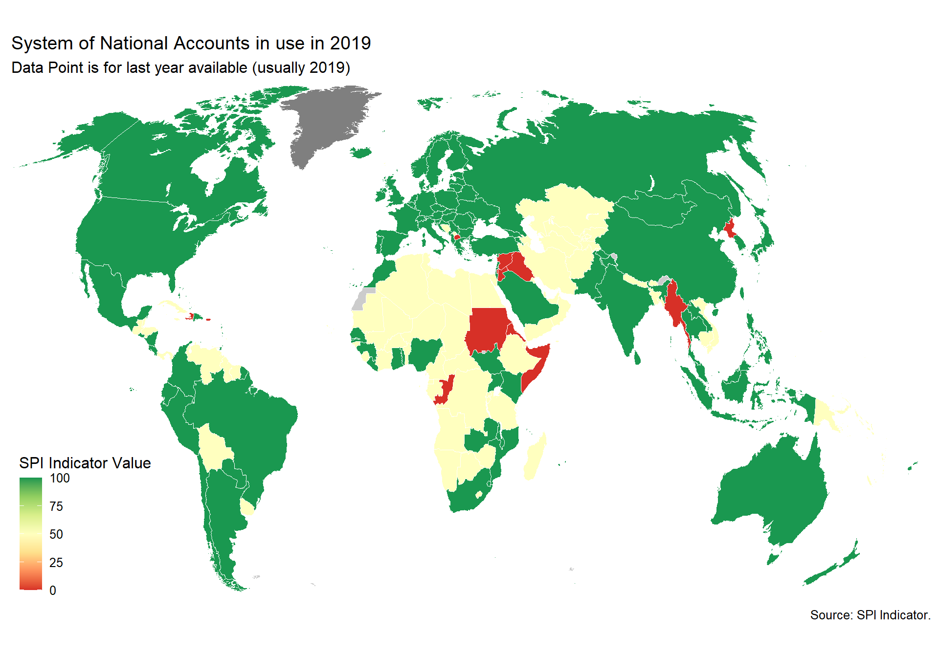
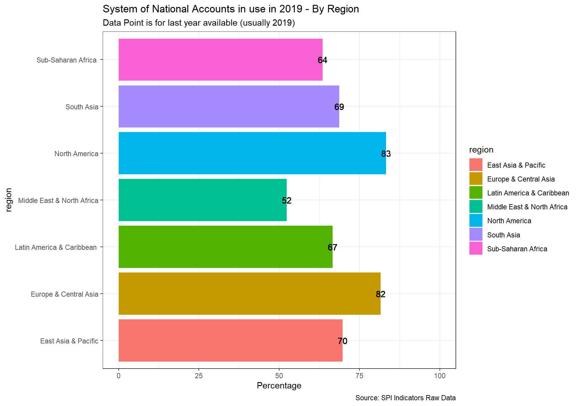
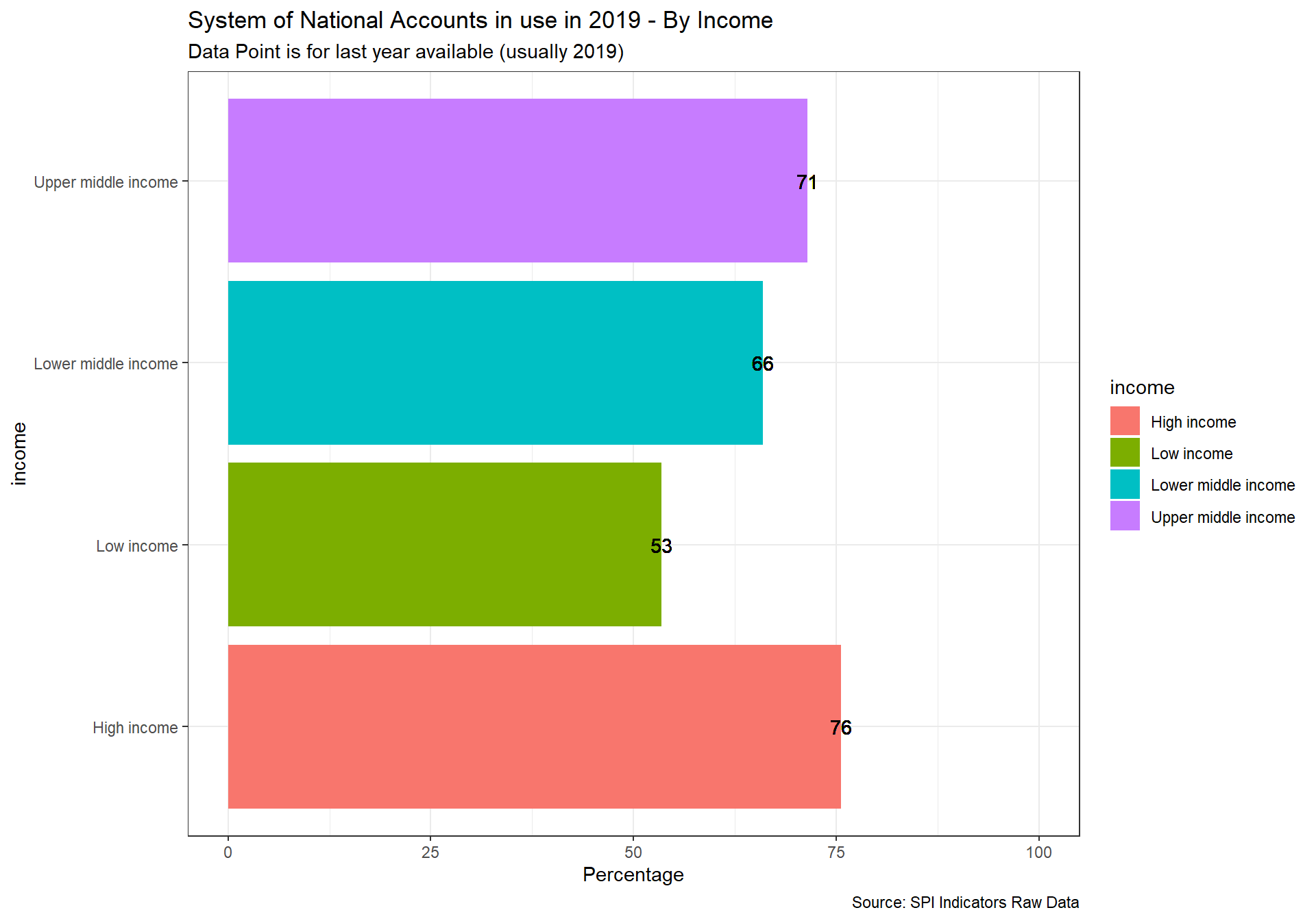
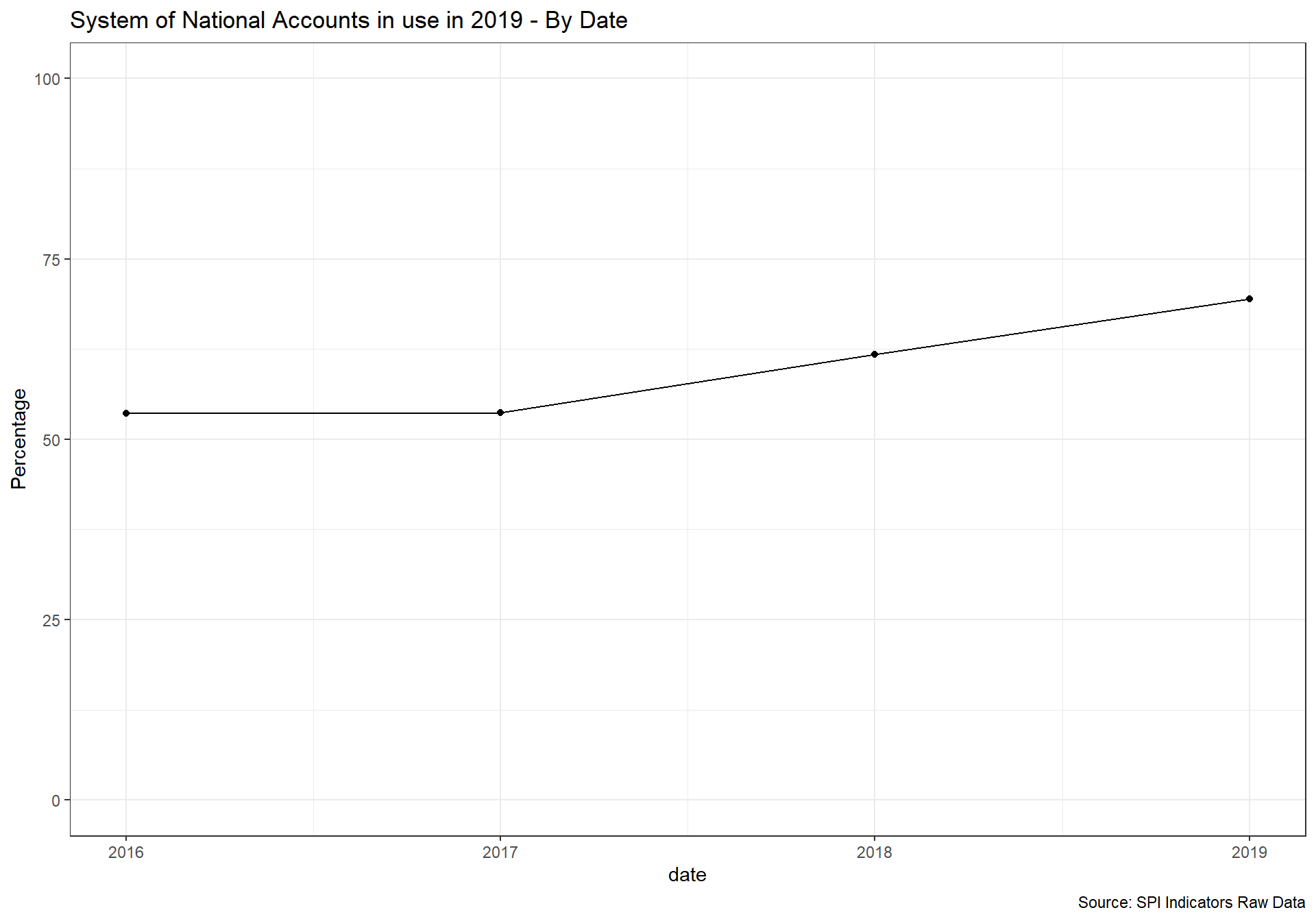
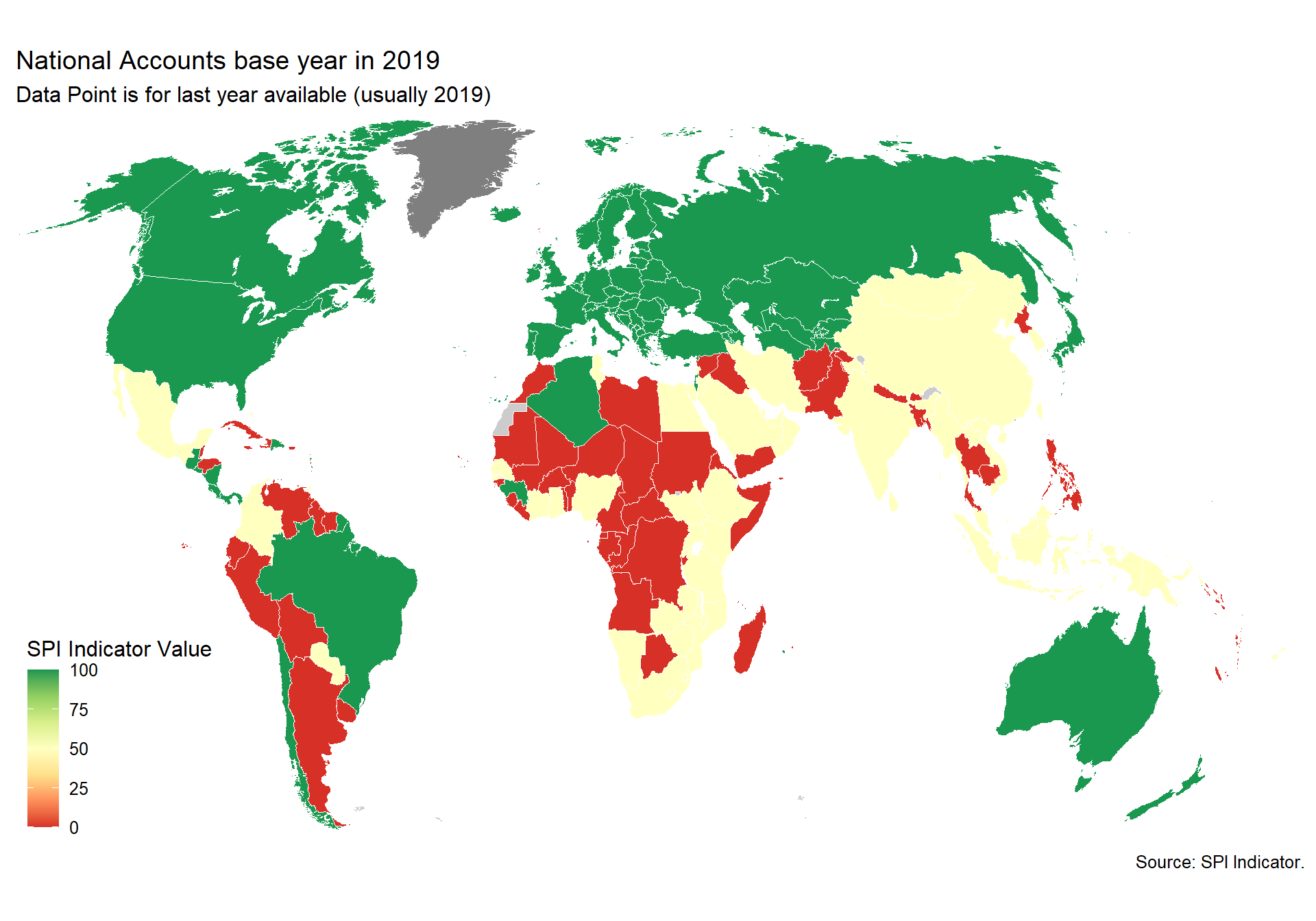
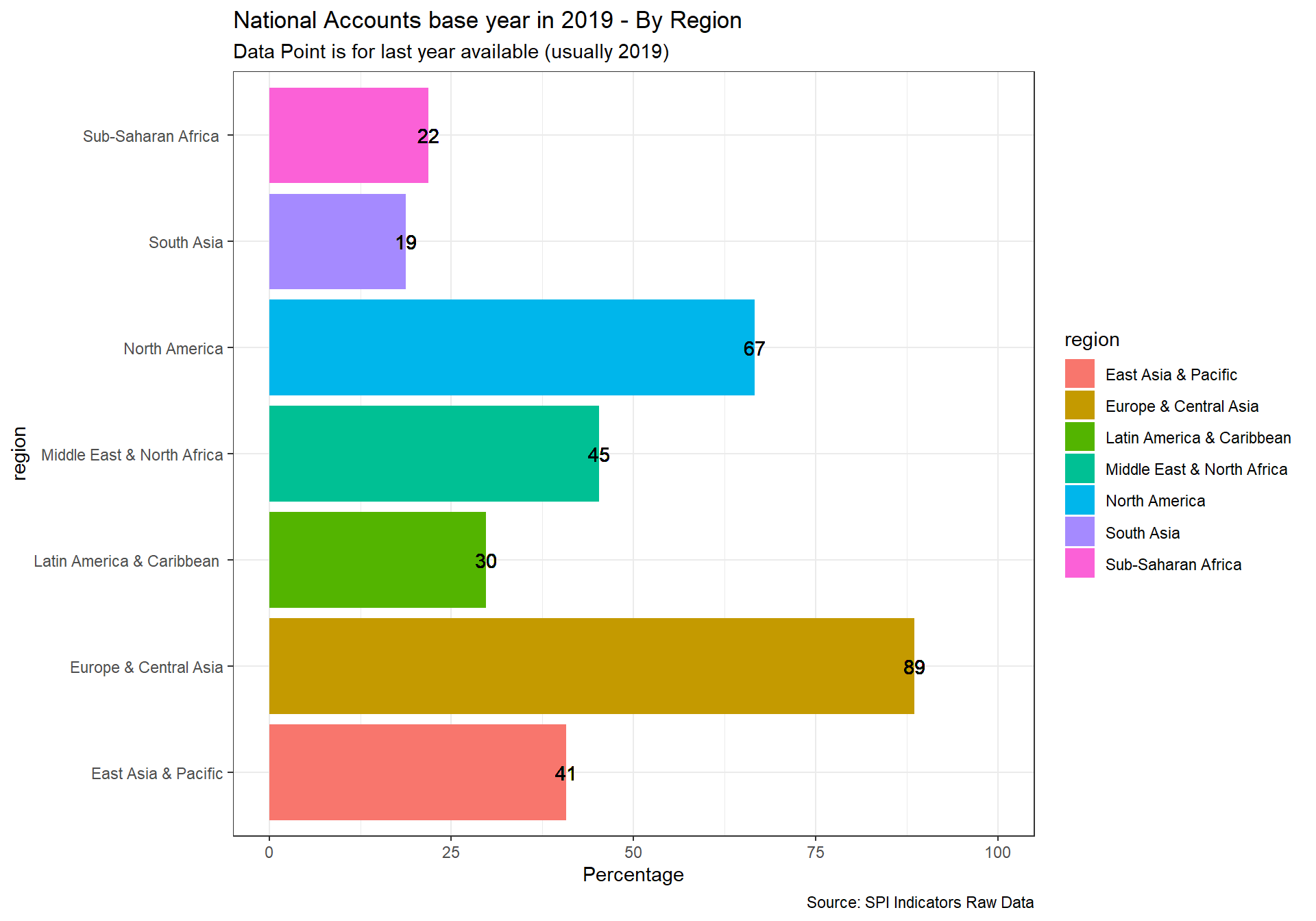
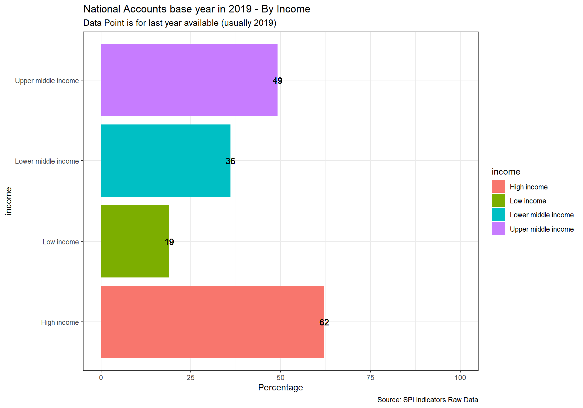
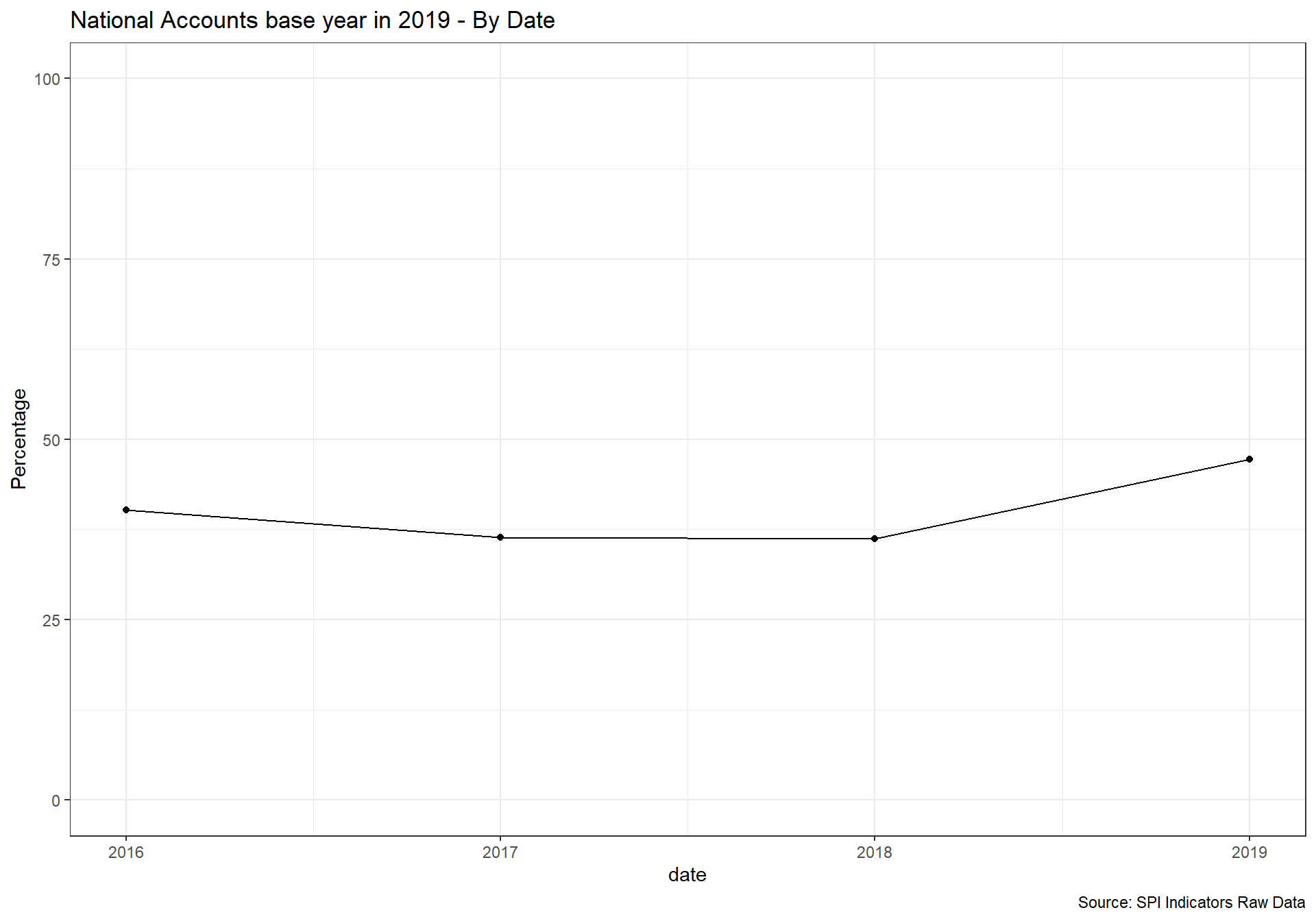
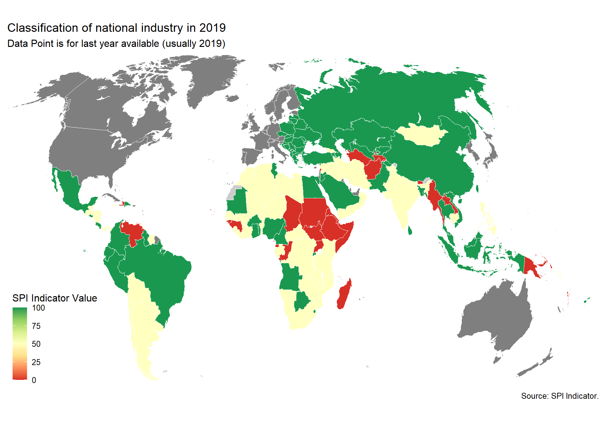
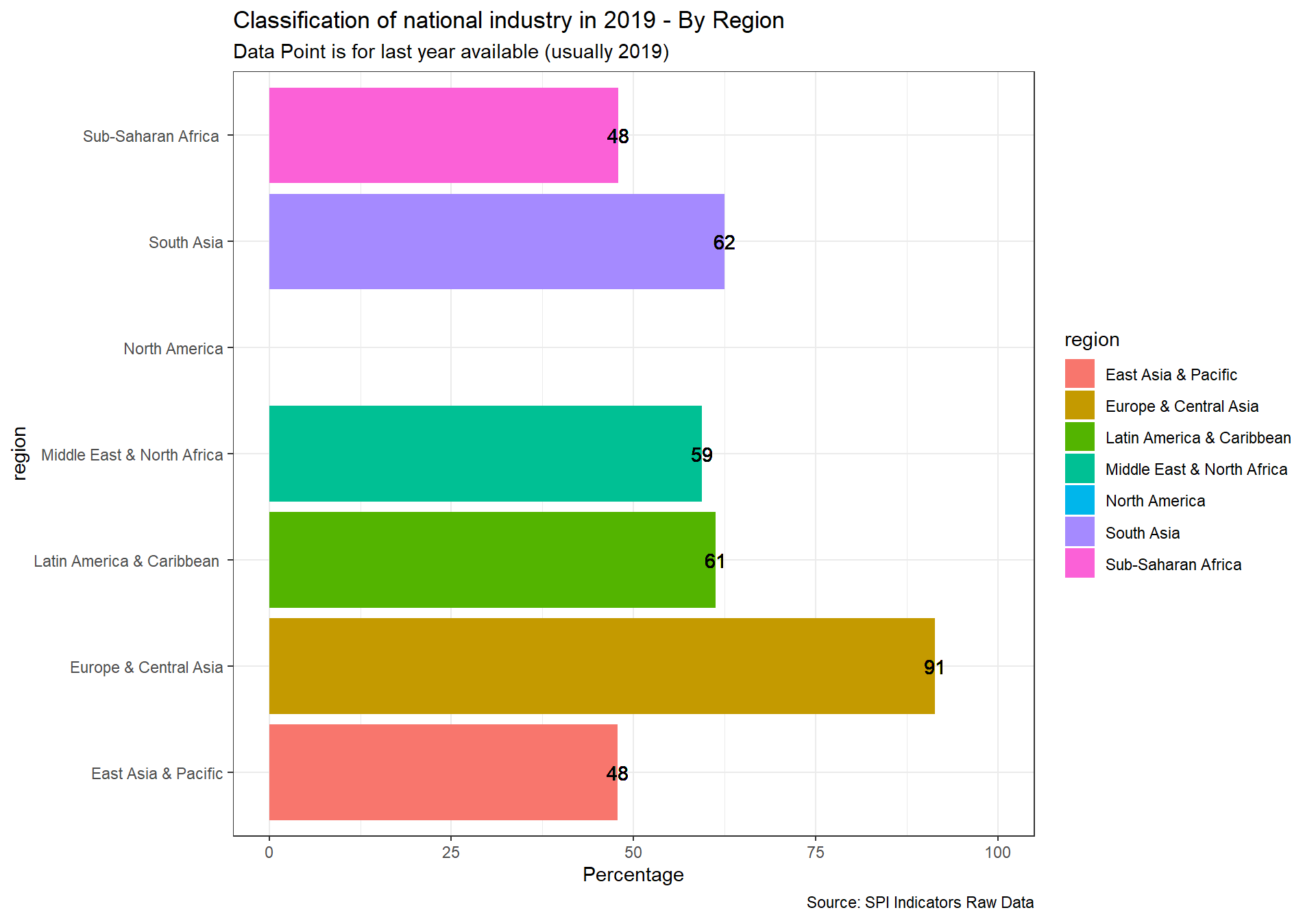
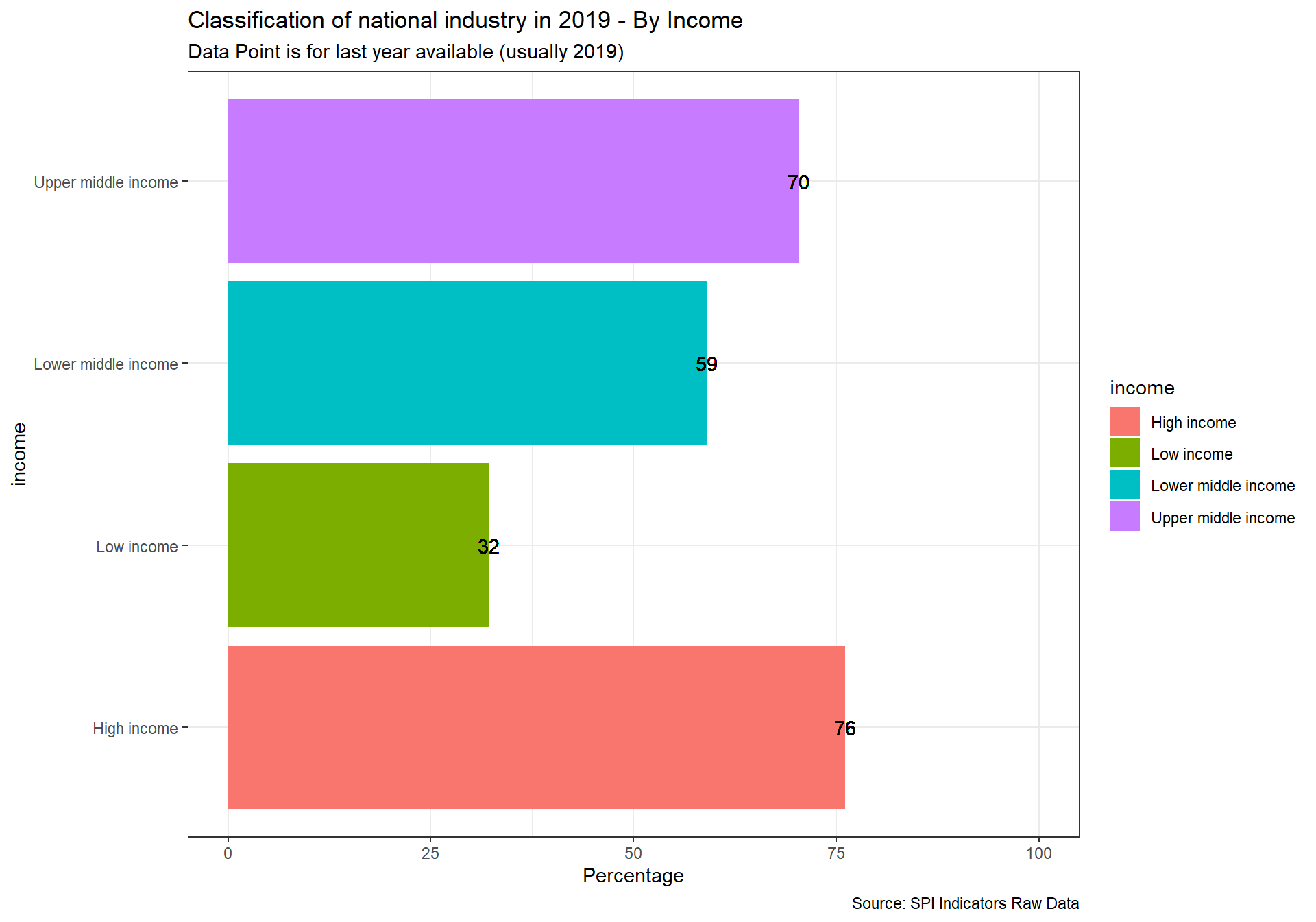
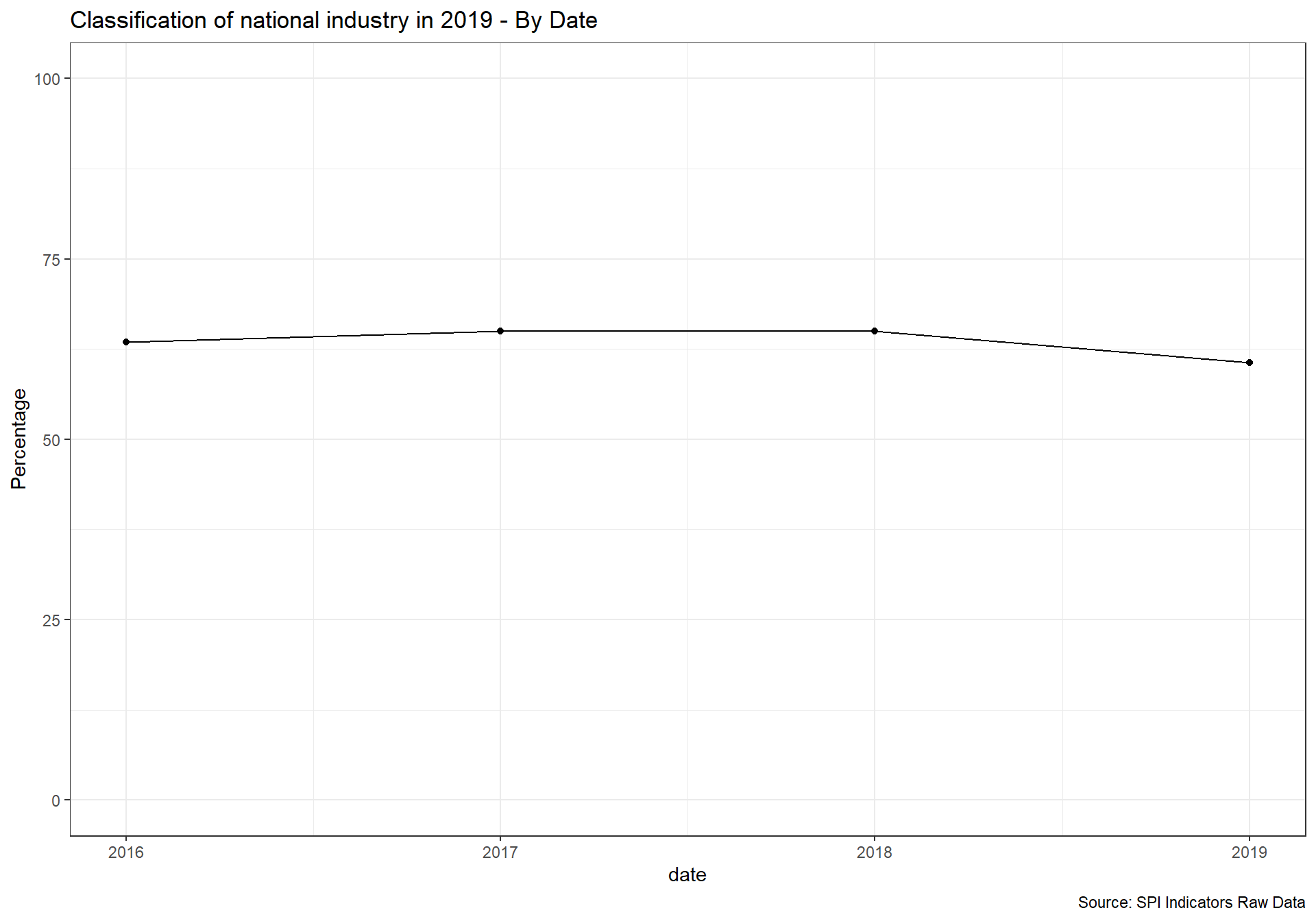
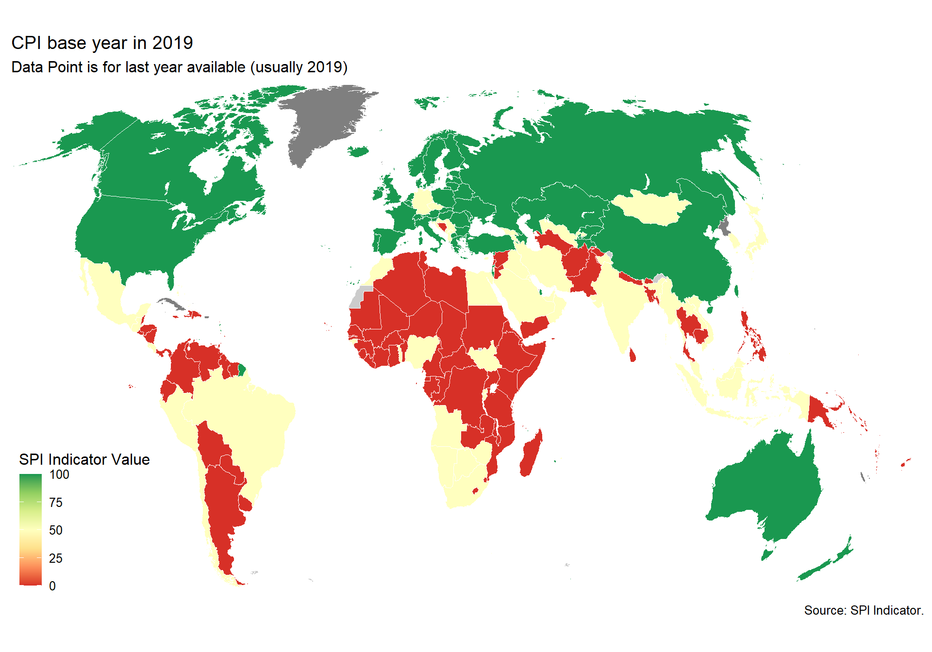
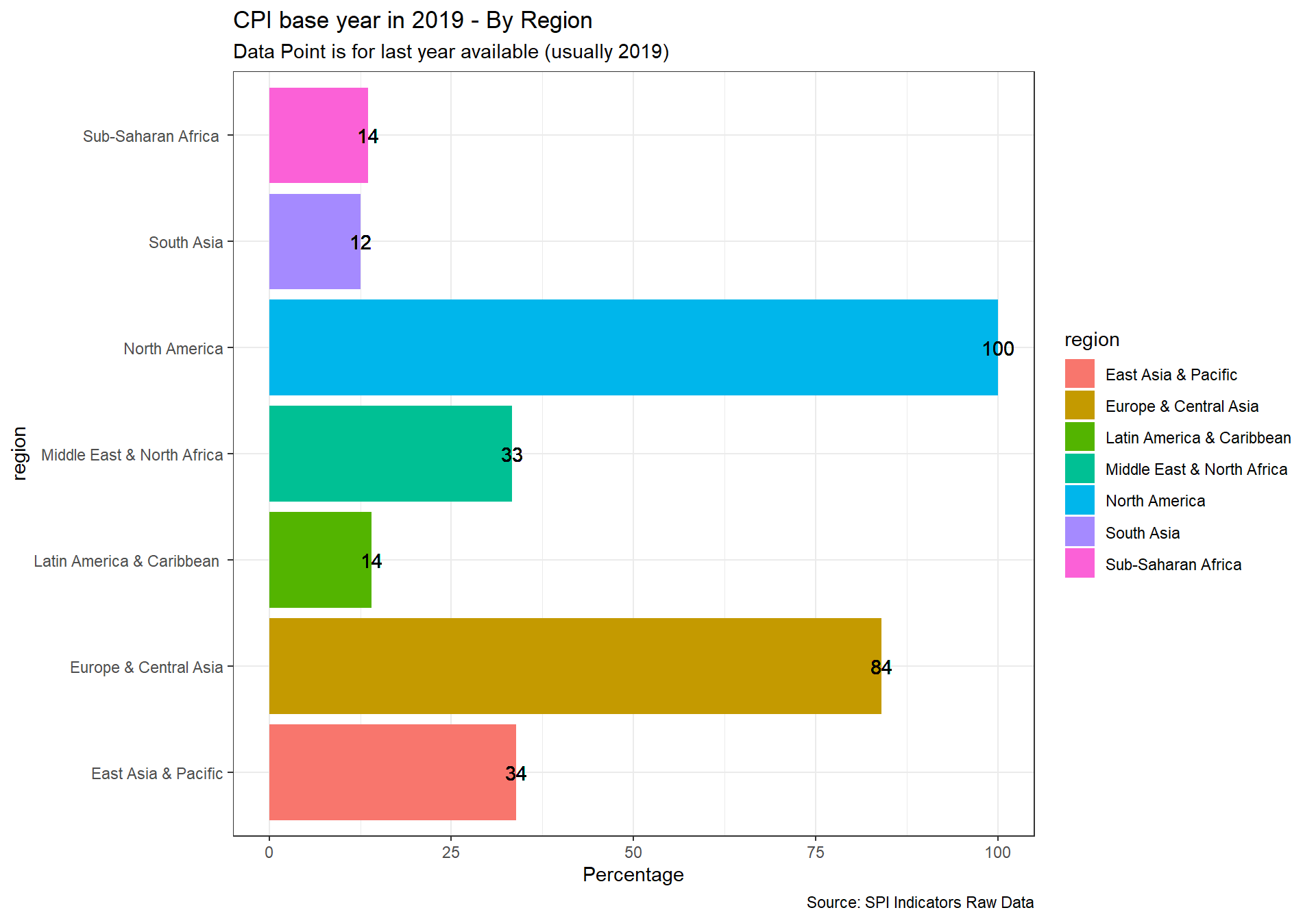
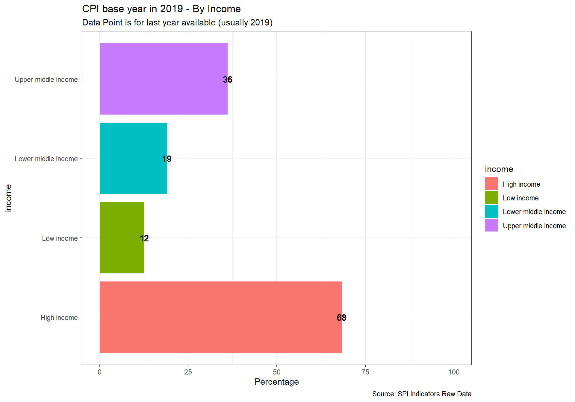
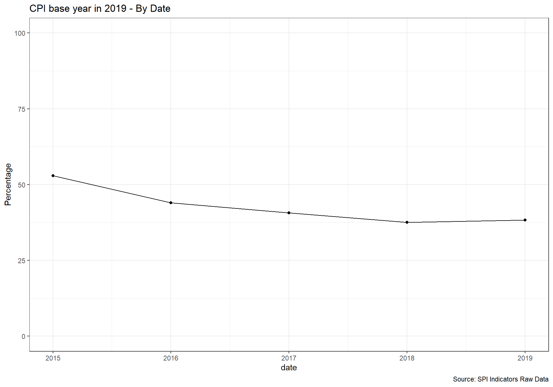
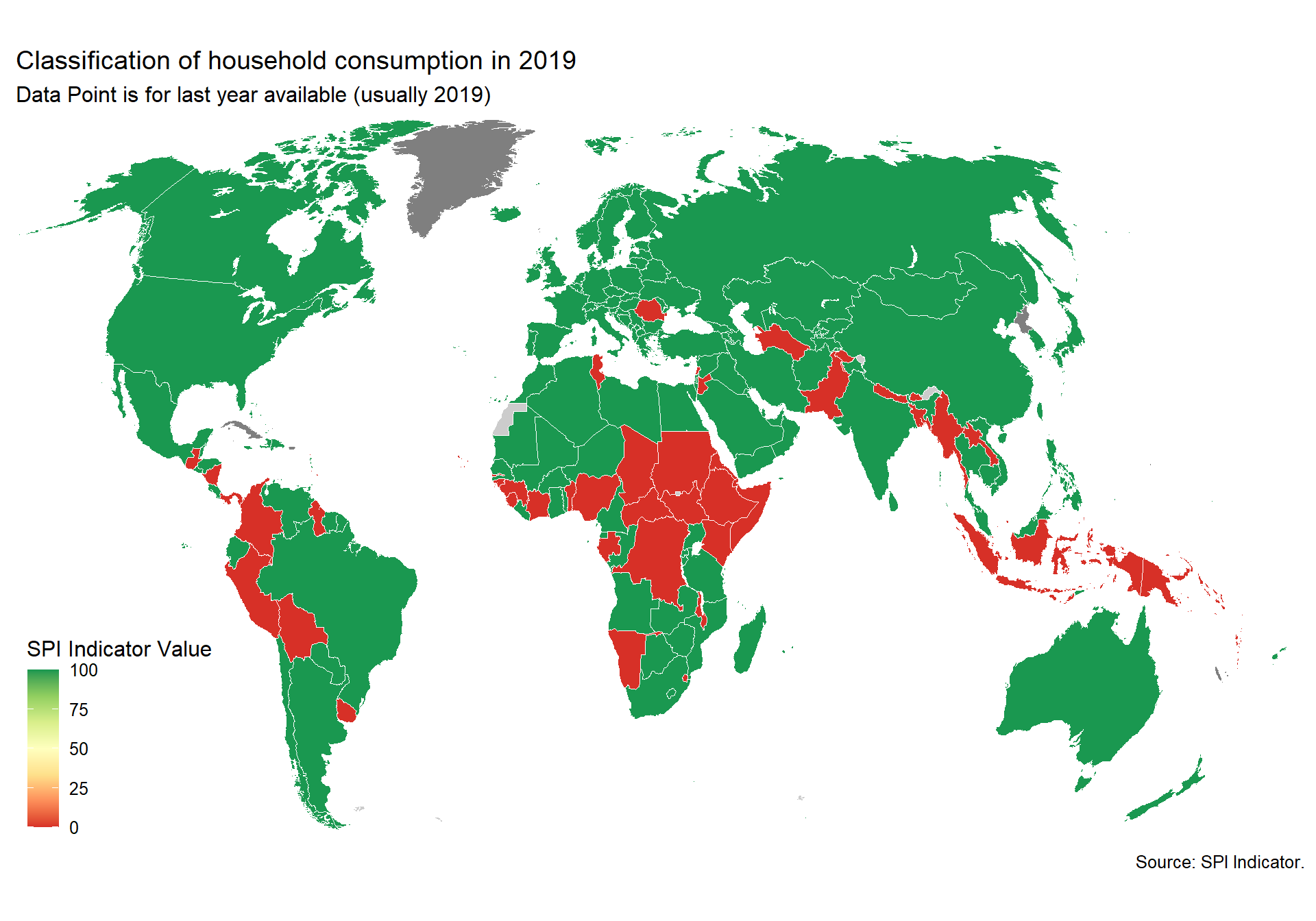
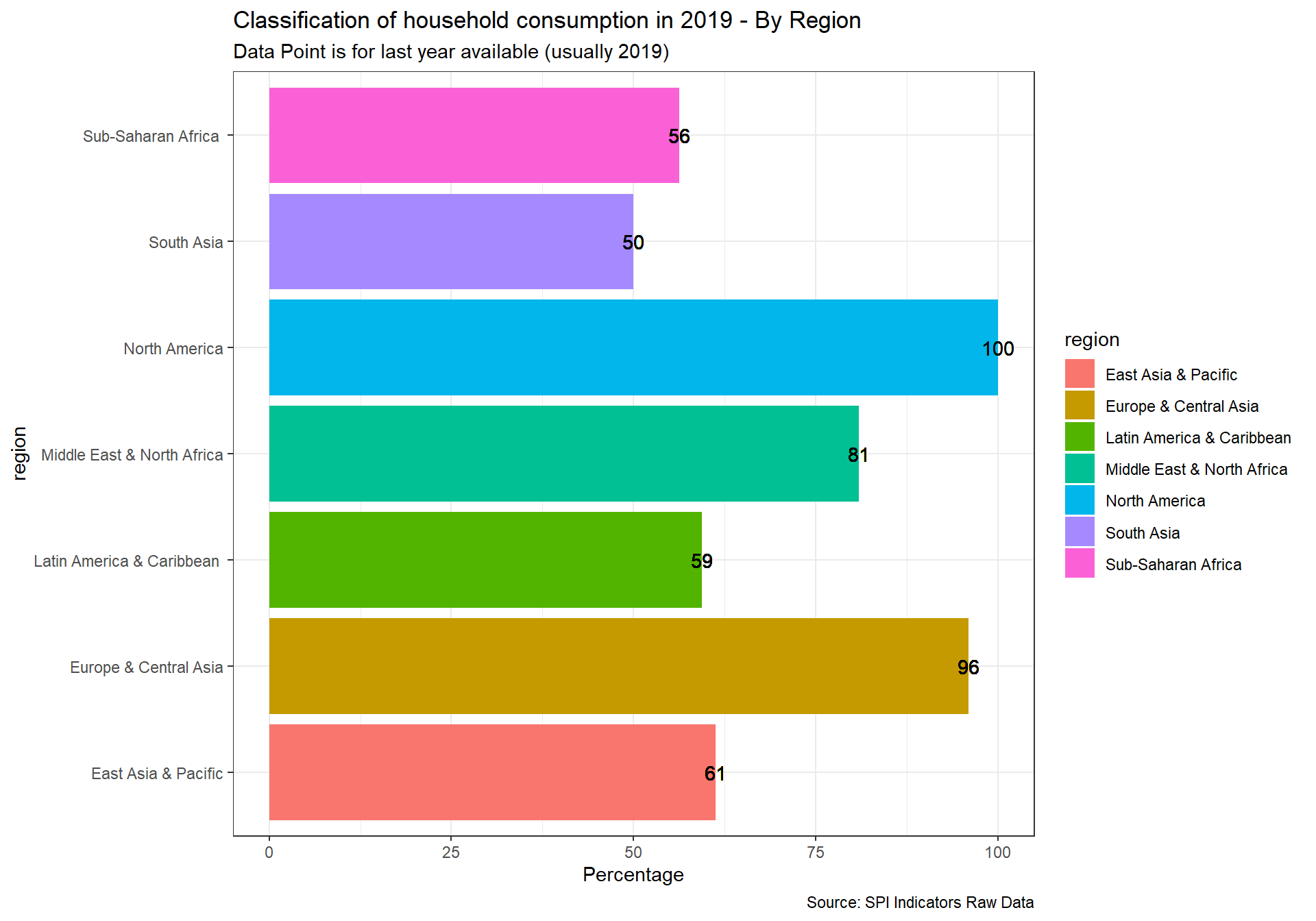
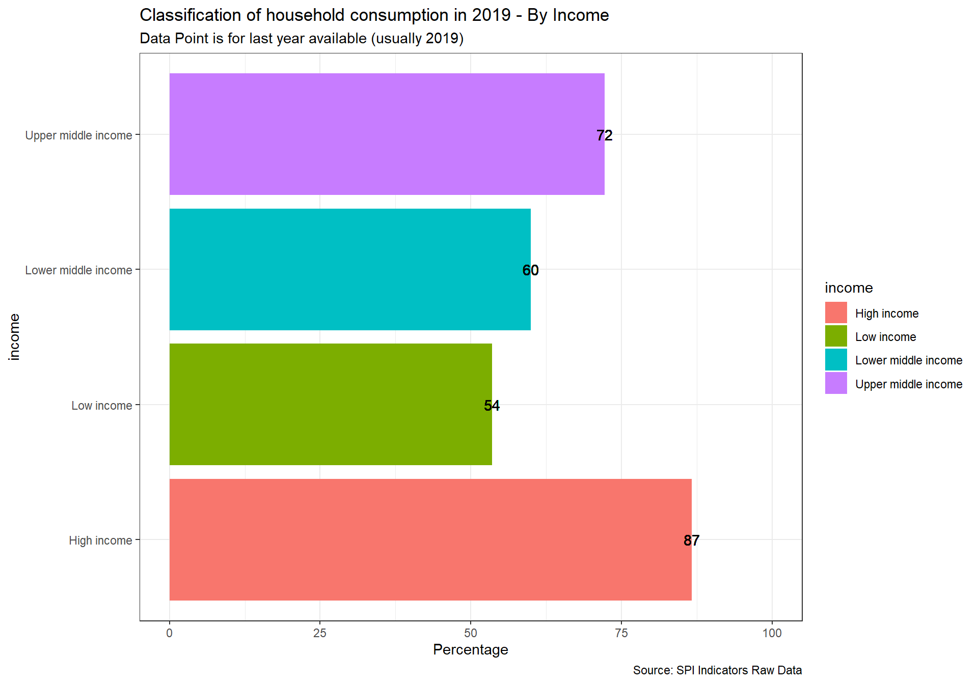
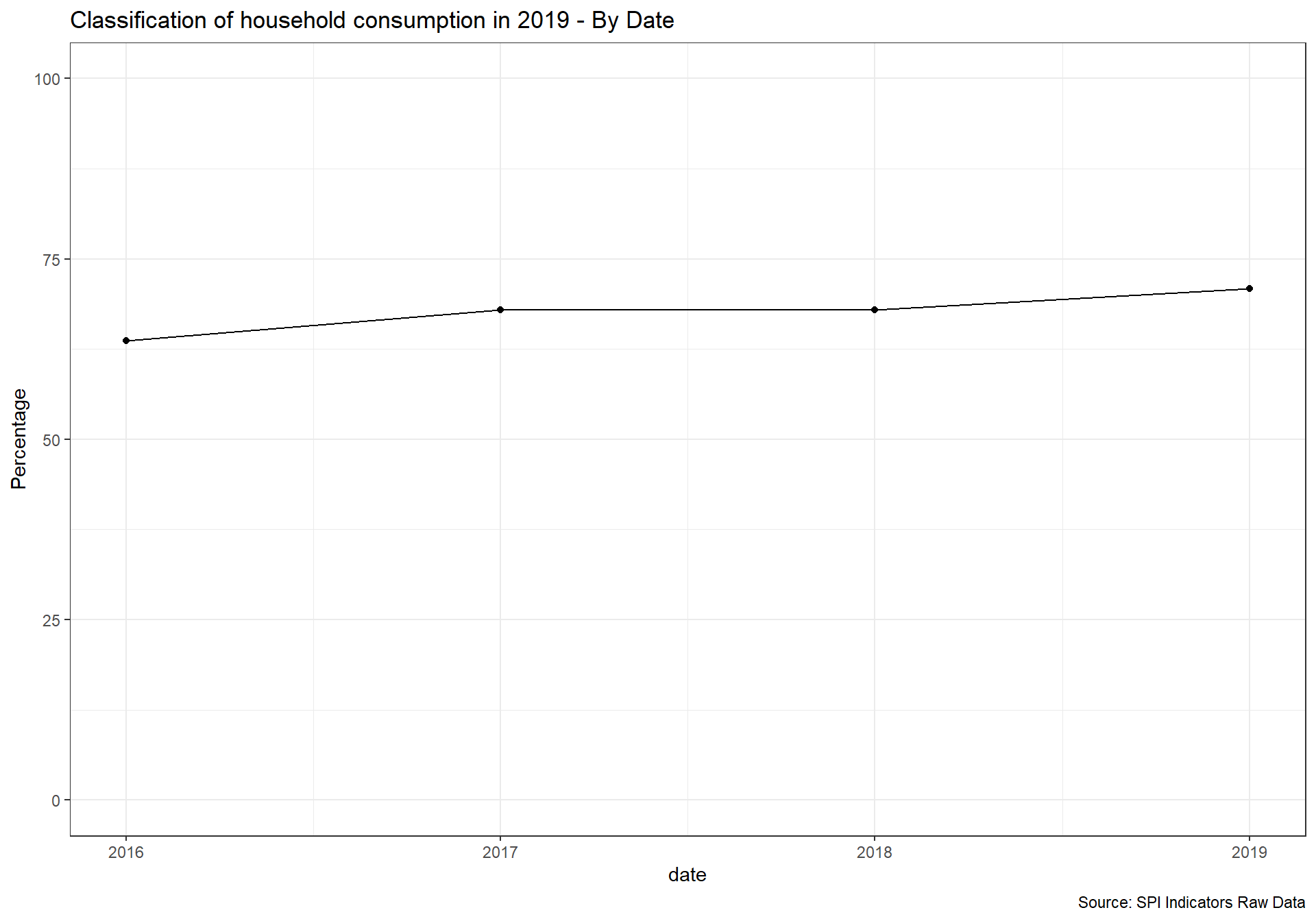
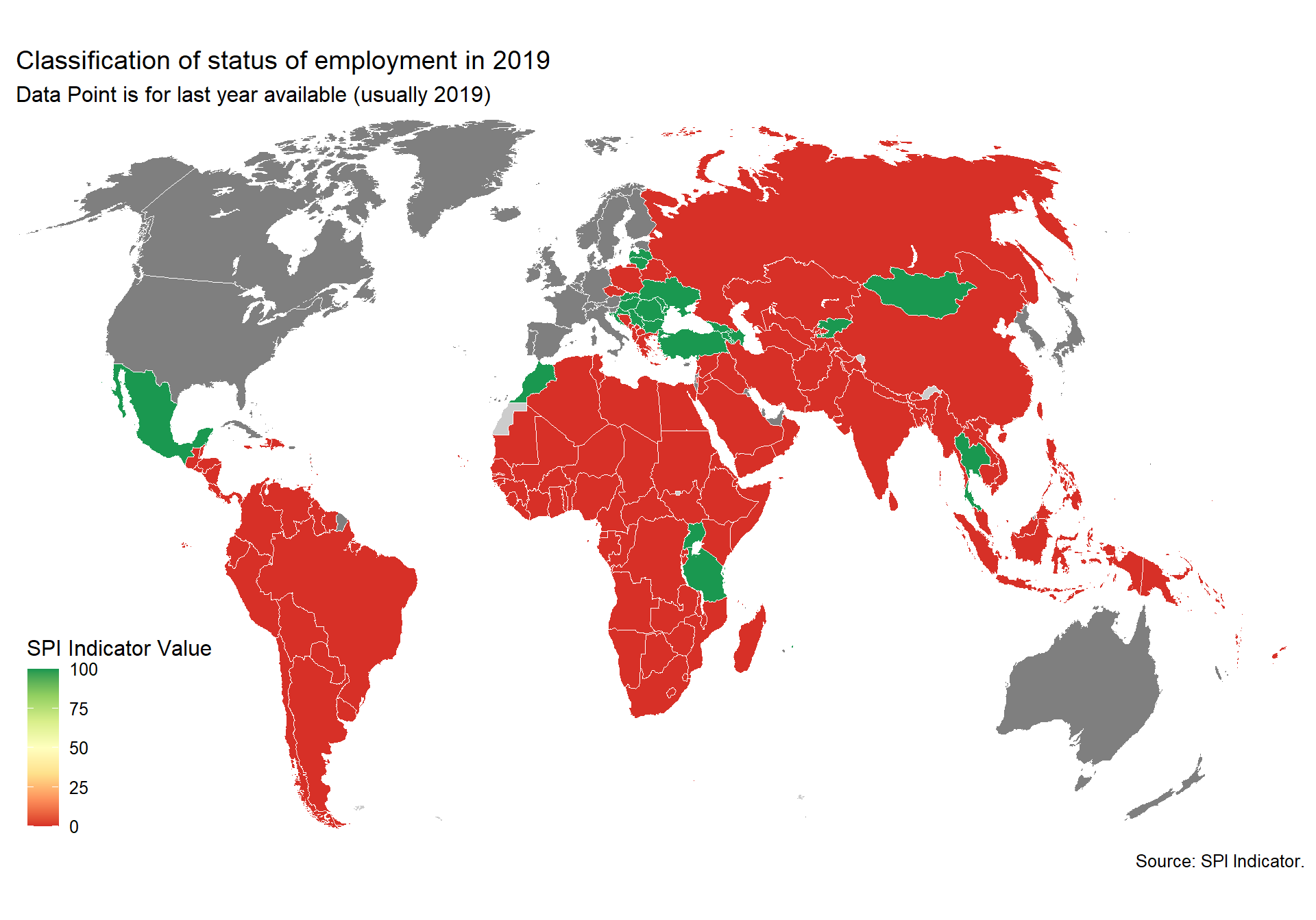
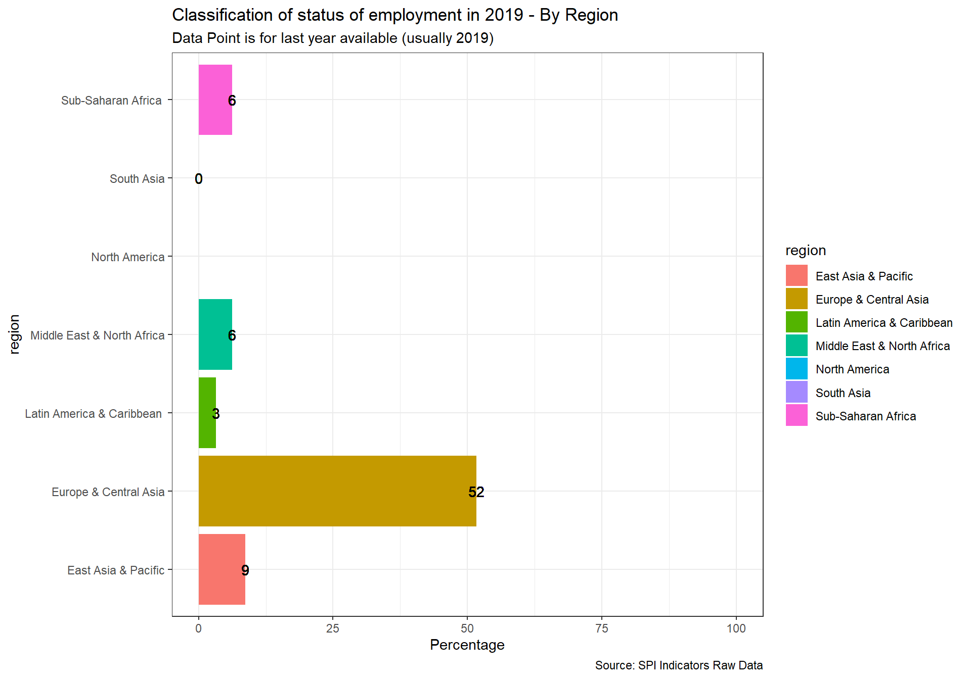
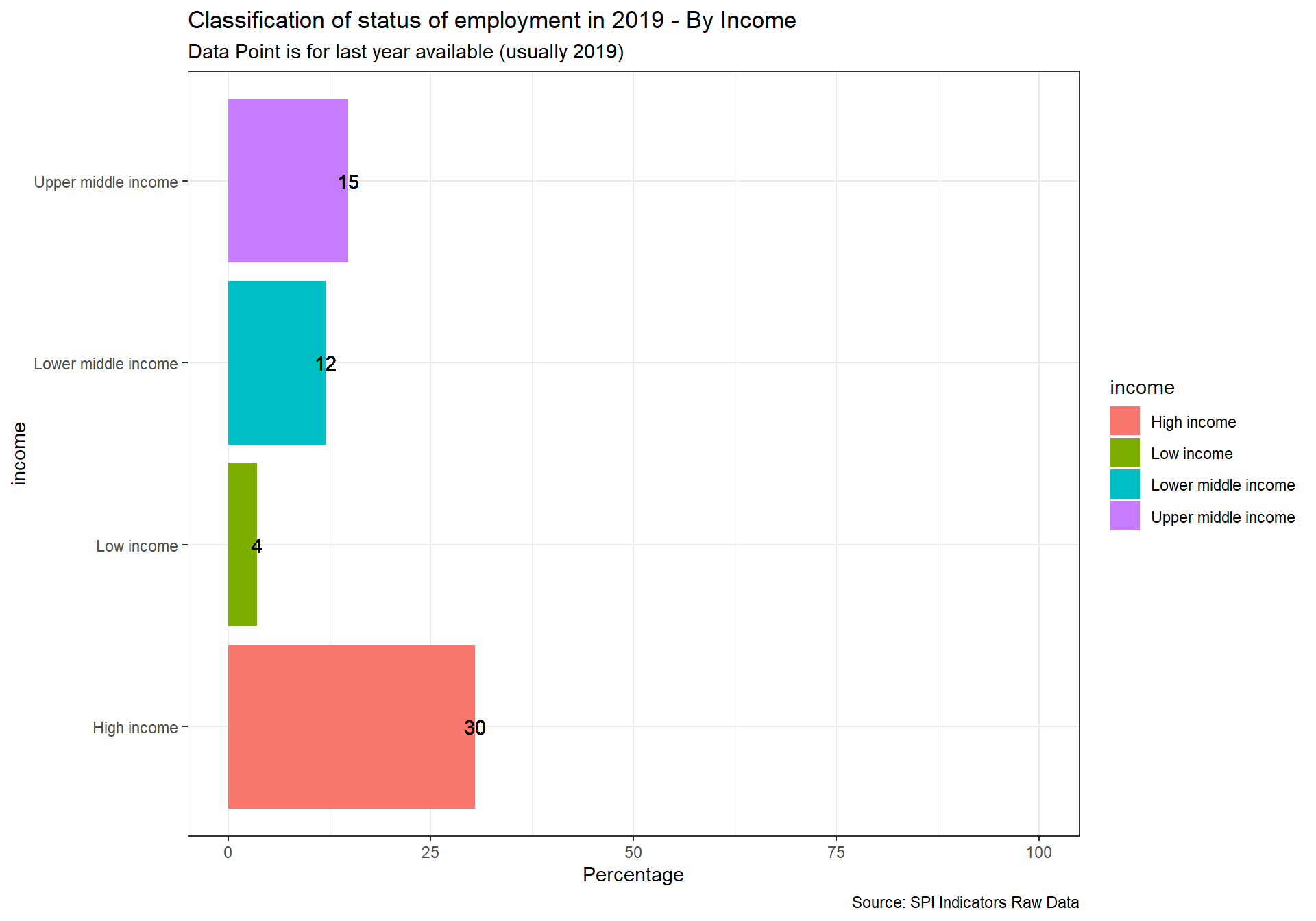
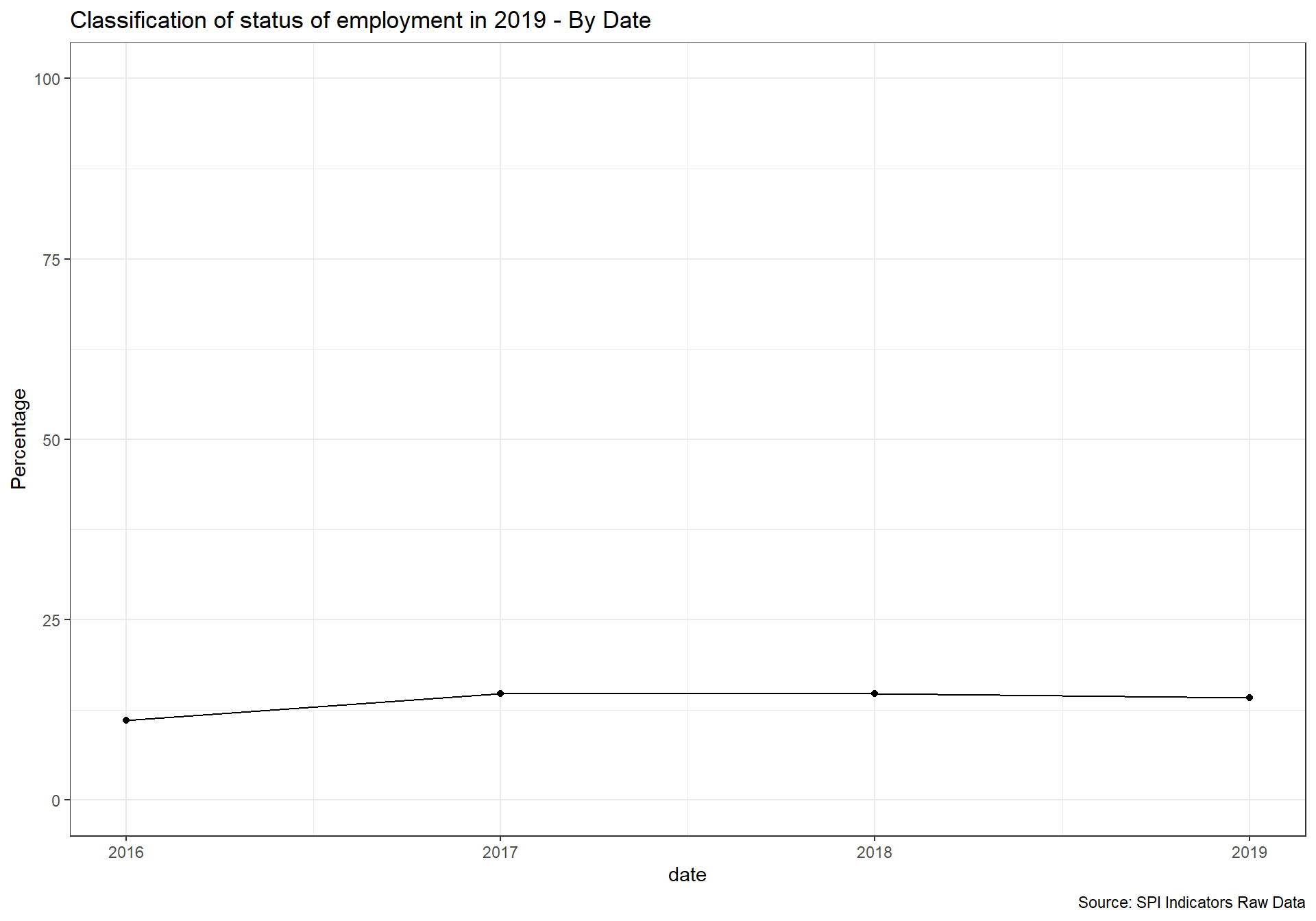
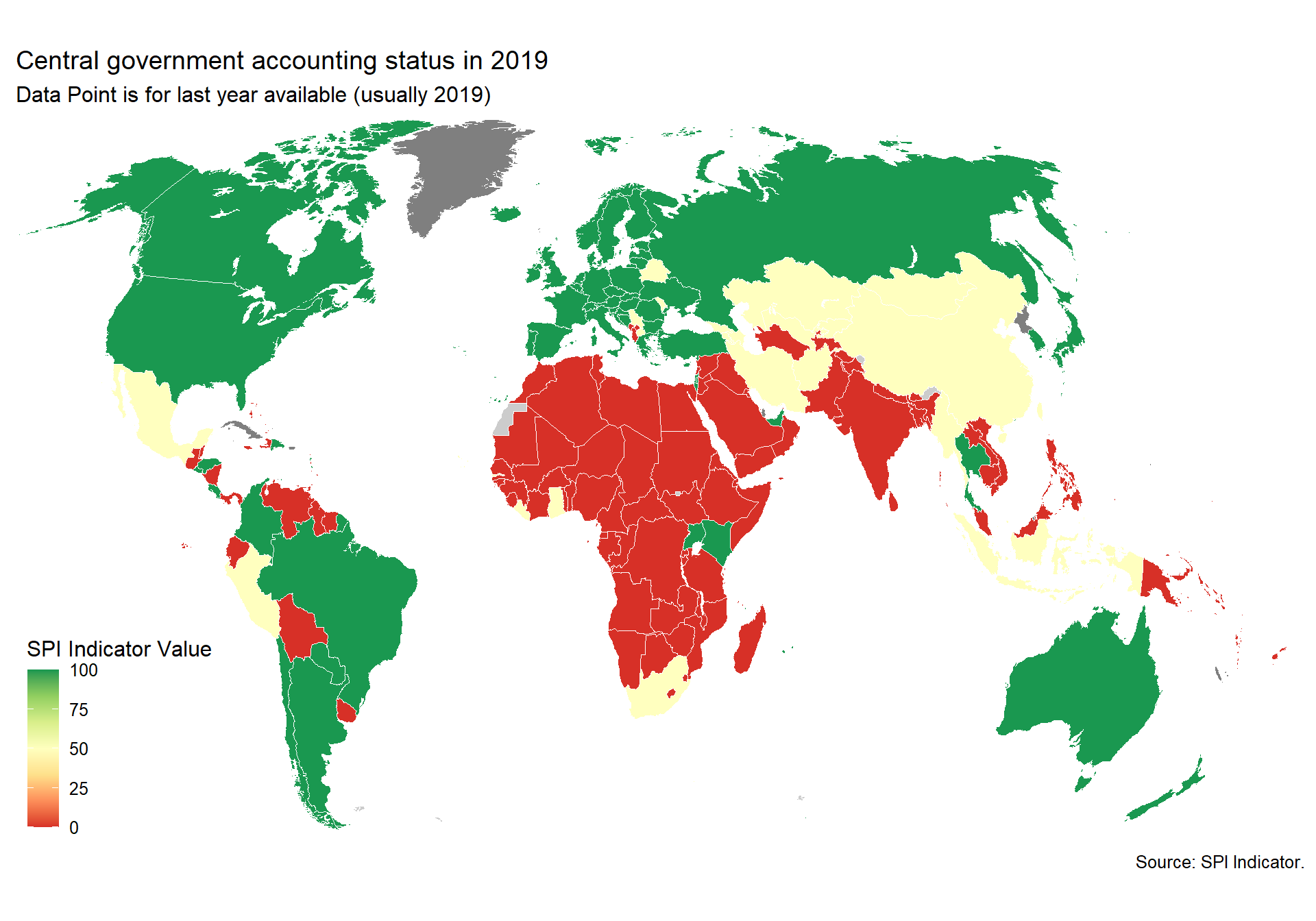
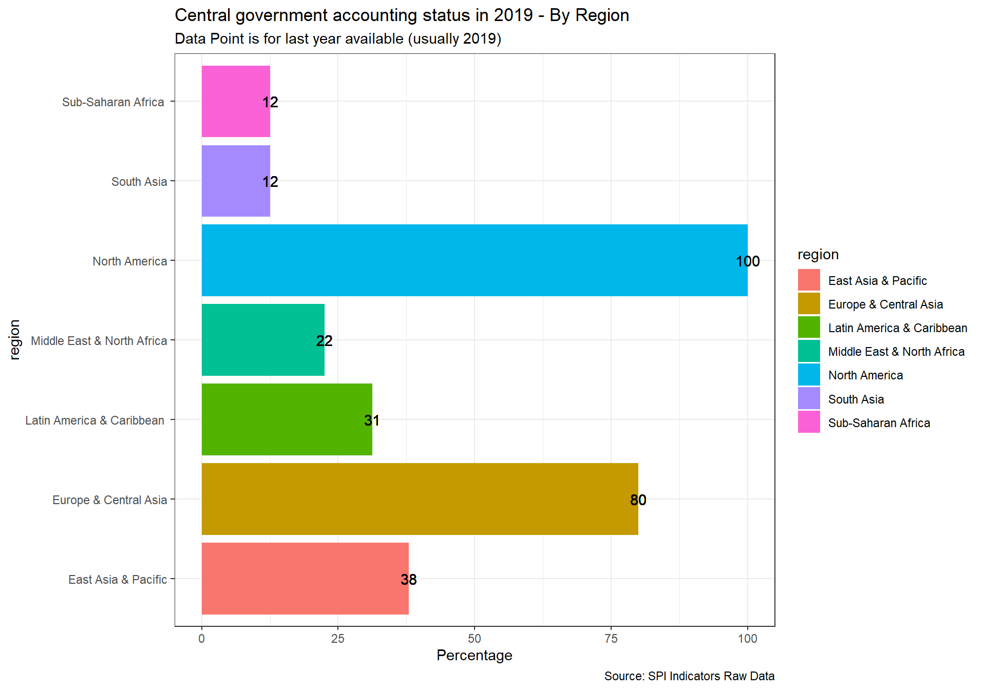
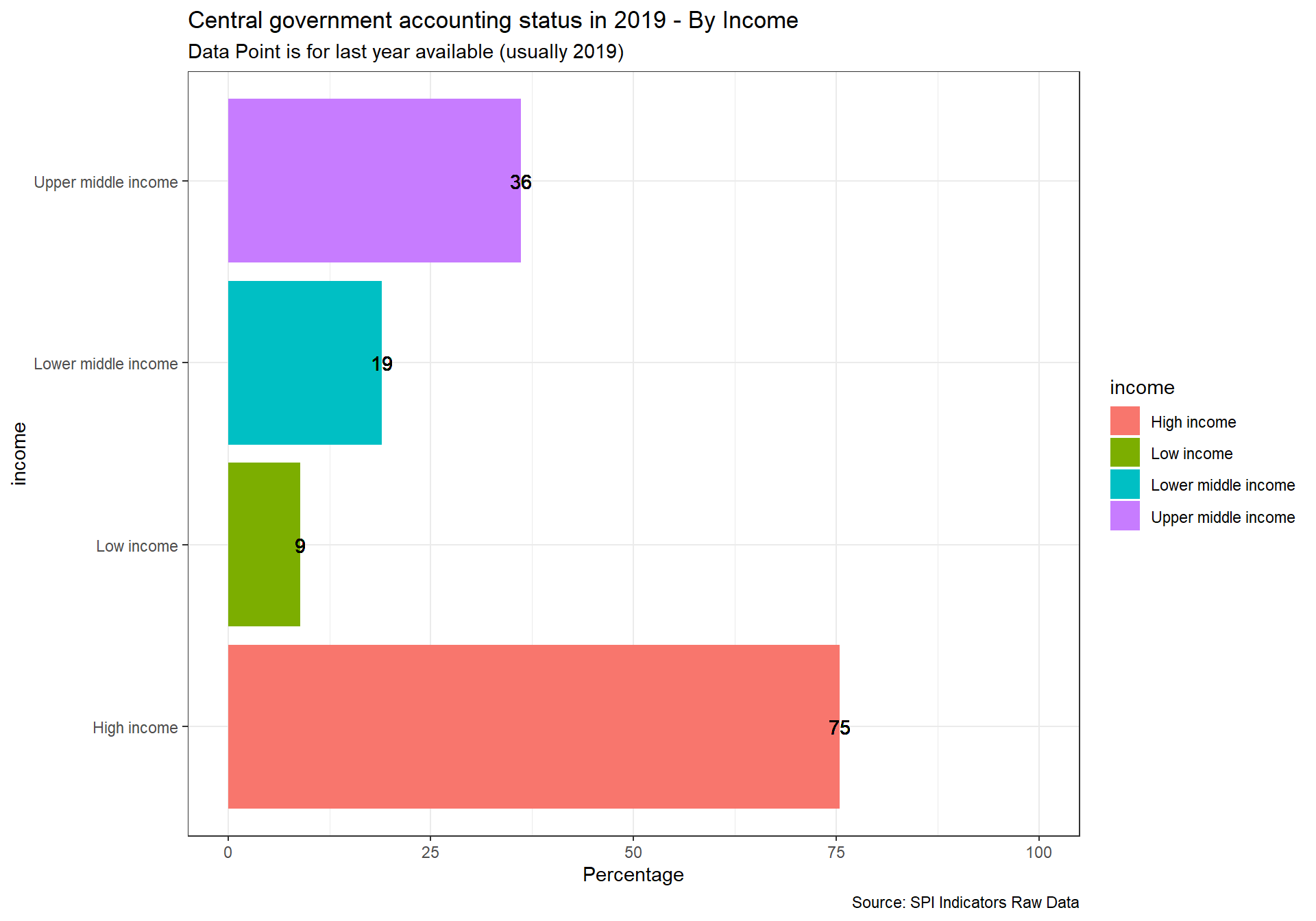

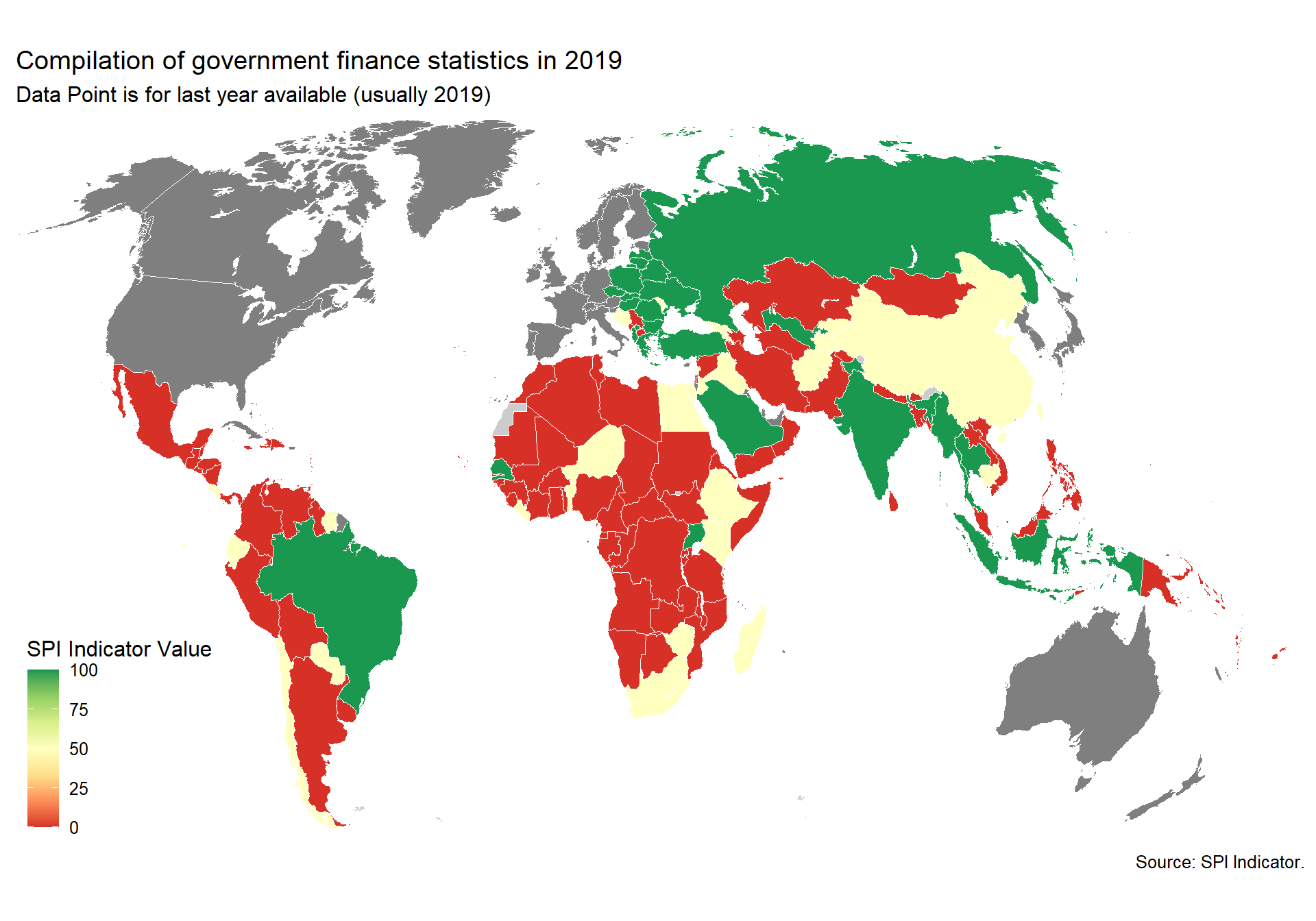
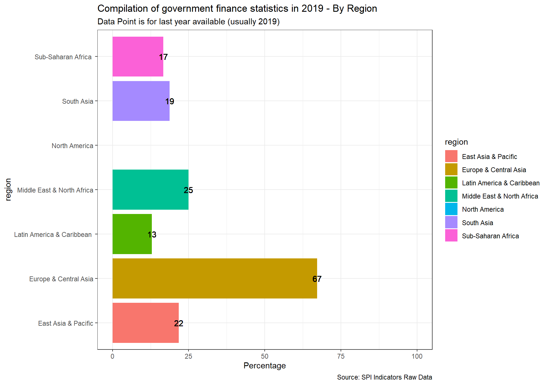
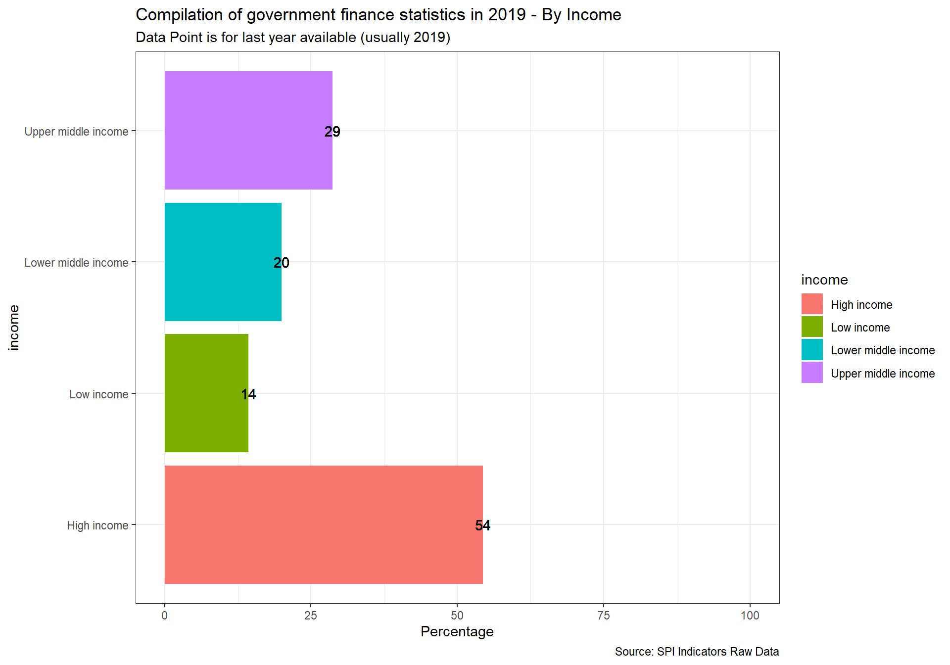
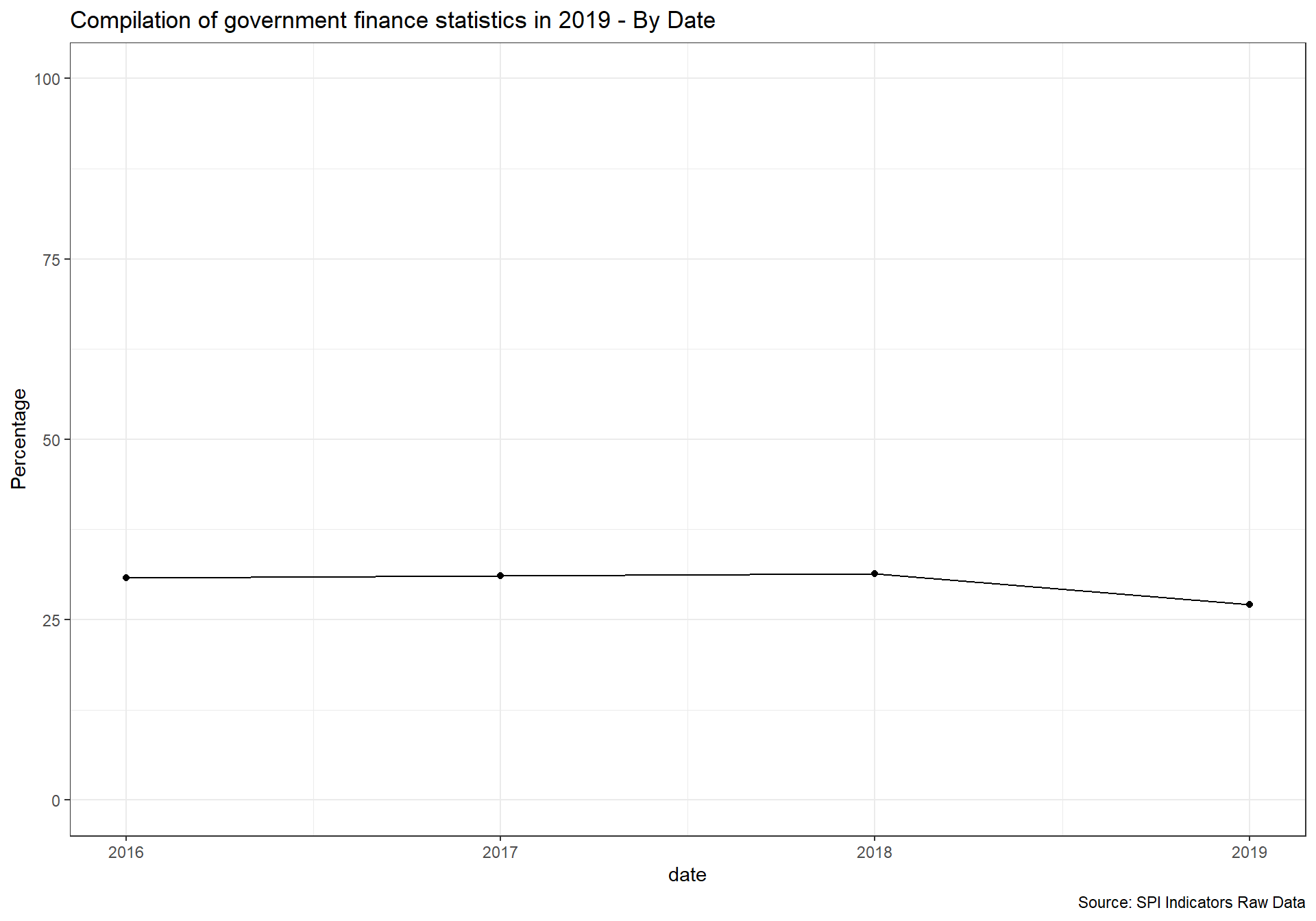


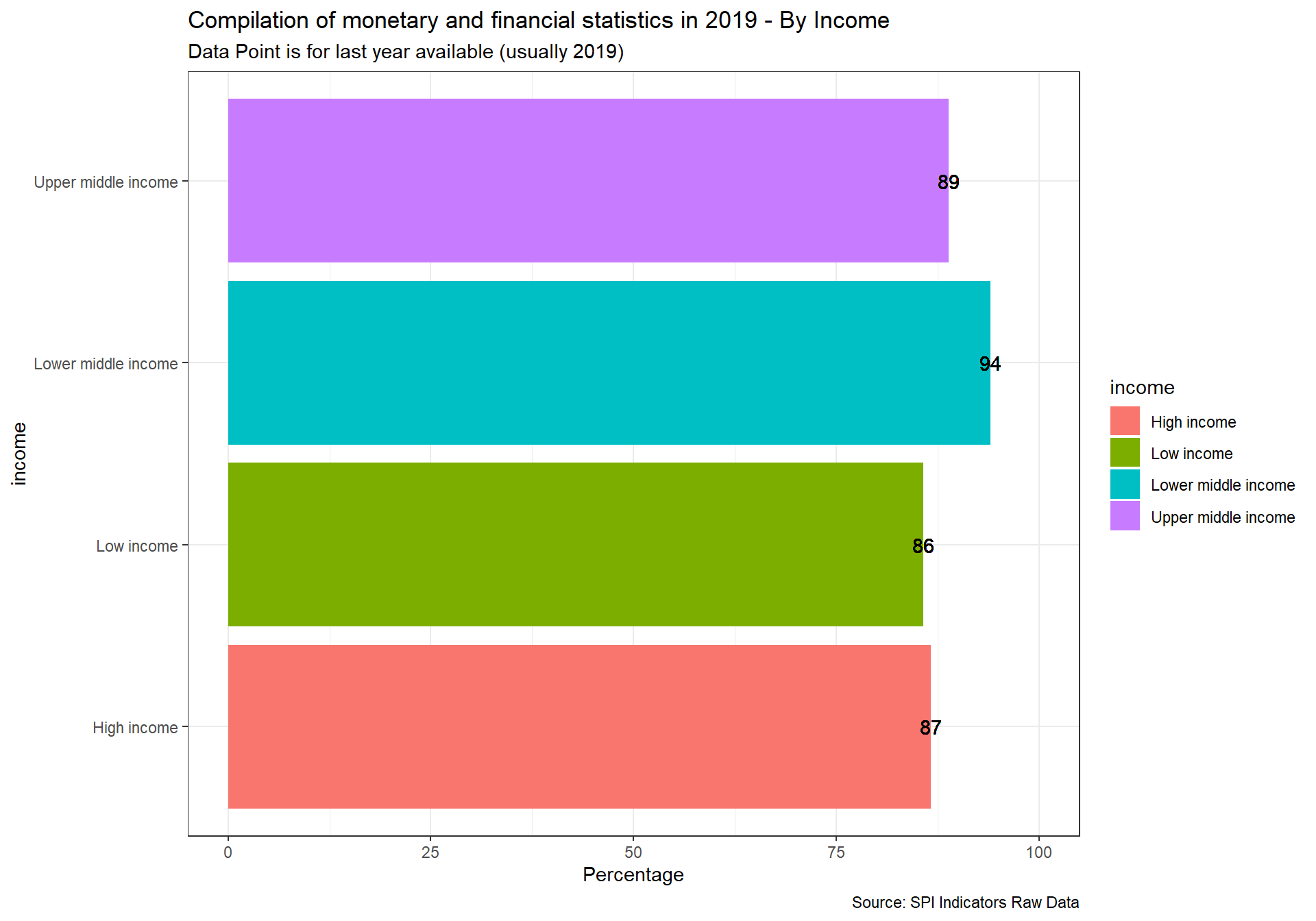
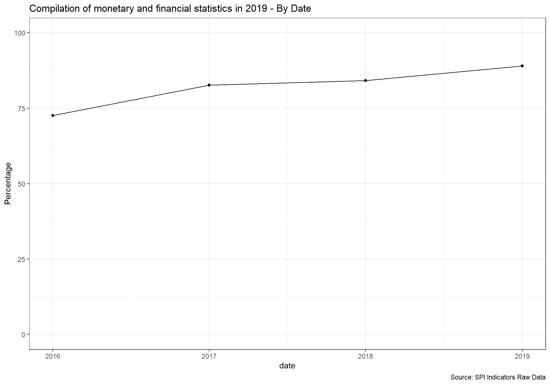
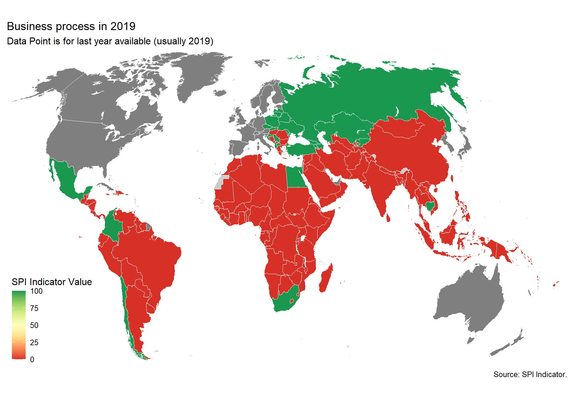
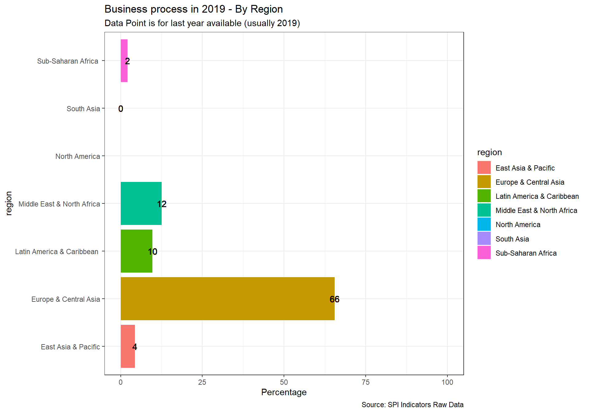
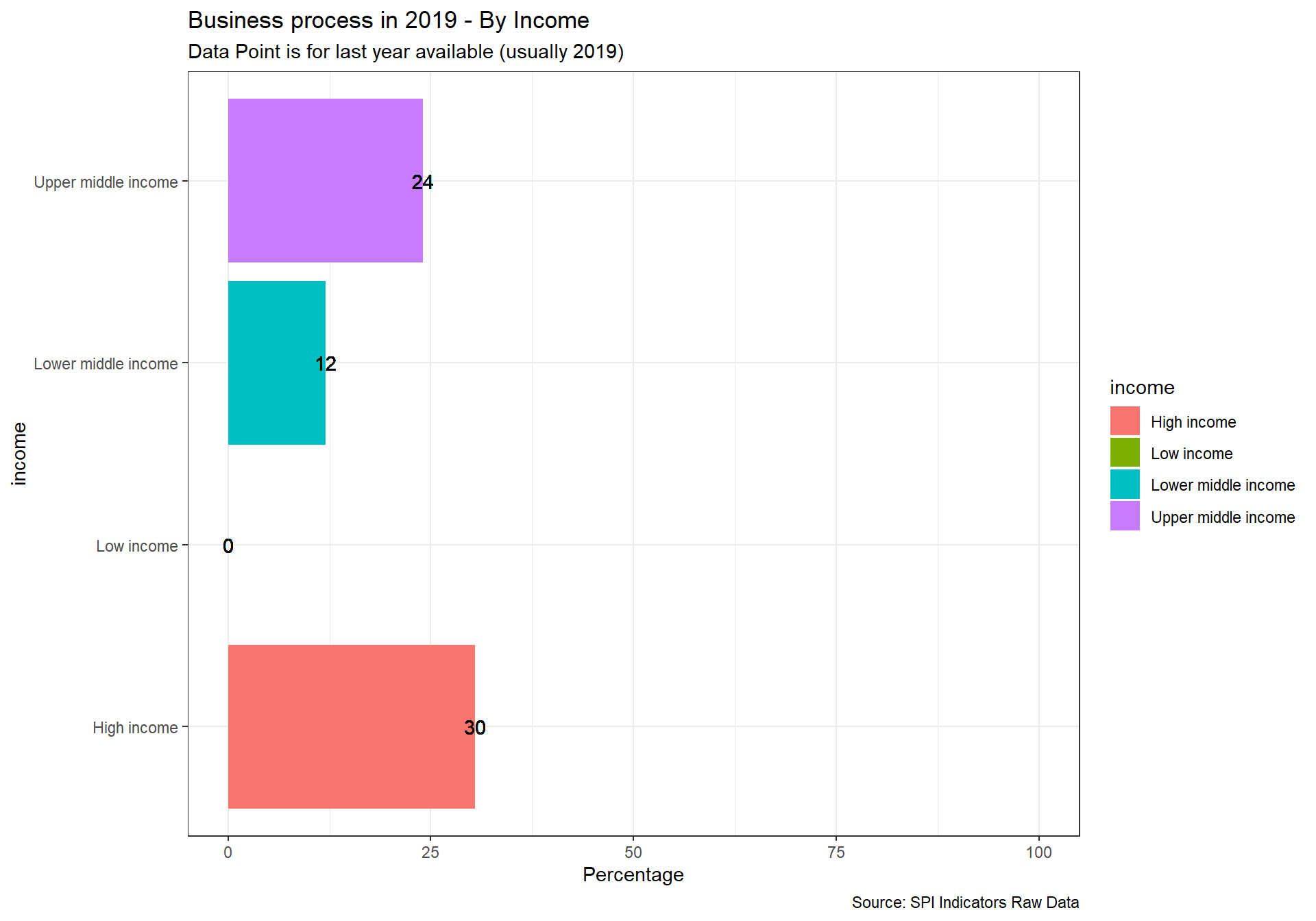
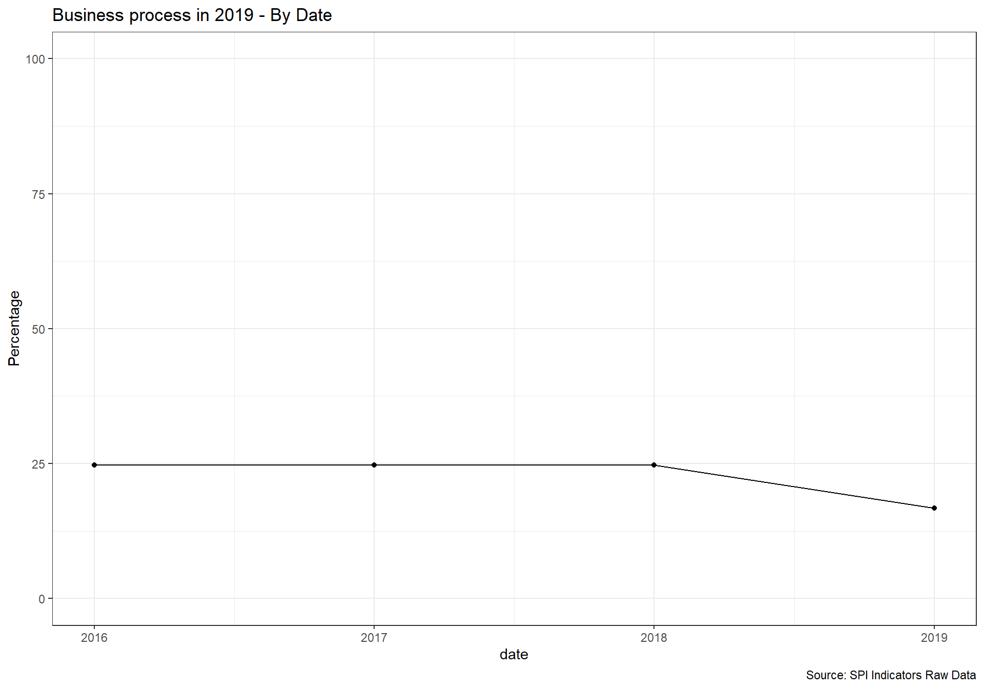
2.5.3 Indicator 5.3: skills
This indicator assesses the systematic use of statistical knowledge with statistical terms and indicators in national policy documents. It is a composite indicator consisting of 4 sub-indices that aim to reflect the relevance of statistical evidence. It comprises four main dimensions: i) Basic consideration; ii) Diagnosis and quantification; iii) Statistical Analysis; iv) Disaggregation.
Score ranges from 0 to 100. The score is the weighted sum of each of the four components’ scores, whose relative weight is reported in brackets: i) Basic Consideration (25%); ii) Diagnosis and quantification (24%); iii) Statistical Analysis (22%); iv) Disaggregation (29%).
The source is Paris 21. Data accessed on August 6, 2020 from https://statisticalcapacitymonitor.org/indicator/127
Not included because of lack of established methodology or suitable data sources.
#read in csv file.
D5.3_DISK <- read_csv(file = paste(raw_dir, "5.3_DISK","5.3_DISK.csv", sep="/" )) %>%
  as_tibble(.name_repair = 'universal') %>%
  transmute(
    country=Country,
    date=Year,
    SPI.D5.3.DISK=Data.Value
  ) %>%
    mutate(country=case_when(
    country=="Bahamas" ~ "Bahamas, The",
    country=="Bolivia (Plurinational State of)"   ~  "Bolivia"   ,
    country=="Côte d'Ivoire"  ~  "Cote d'Ivoire"                ,
    country=="Democratic Republic of the Congo"  ~ "Congo, Dem. Rep."  ,
    country=="Congo"  ~ "Congo, Rep."        ,
    country=="Curacao"  ~  "Curacao"       ,
    country=="Czechia"   ~  "Czech Republic"     ,
    country=="Egypt"  ~ "Egypt, Arab Rep."        ,
    country=="Micronesia (Federated States of)"  ~ "Micronesia, Fed. Sts."  ,
    country=="United Kingdom"   ~  "United Kingdom"    ,
    country=="Gambia"    ~  "Gambia, The"     ,
    country=="Iran (Islamic Republic of)"  ~ "Iran, Islamic Rep." ,
    country=="Kyrgyzstan"   ~  "Kyrgyz Republic"   ,
    country=="Republic of Korea"   ~ "Korea, Rep."   ,
    country=="Lao People's Democratic Republic"    ~  "Lao PDR" ,
    country=="Saint Kitts and Nevis "   ~ "St. Kitts and Nevis",
    country=="Saint Lucia"   ~ "St. Lucia",
    country=="Republic of Moldova"   ~  "Moldova"   ,
    country=="Democratic People's Republic of Korea"  ~  "Korea, Dem. People’s Rep." ,
    country=="Slovakia"   ~  "Slovak Republic"             ,
    country=="United Republic of Tanzania"   ~  "Tanzania" ,
    country=="United States of America"  ~ "United States"  ,
    country=="Saint Vincent and the Grenadines" ~ "St. Vincent and the Grenadines" ,
    country=="Venezuela (Bolivarian Republic of)"  ~  "Venezuela, RB"   ,
    country=="British Virgin Islands"  ~  "British Virgin Islands" ,
    country=="Viet Nam"  ~ "Vietnam"        ,
    country=="Yemen"  ~ "Yemen, Rep.",
    country=="United Kingdom of Great Britain and Northern Ireland" ~ "United Kingdom",
    TRUE ~ country
  )) %>%
  mutate(RAW.D5.3.DISK=if_else(SPI.D5.3.DISK=='no data',as.character(NA), SPI.D5.3.DISK),
         SPI.D5.3.DISK=if_else(SPI.D5.3.DISK=='no data',as.numeric(NA), as.numeric(SPI.D5.3.DISK))/100) %>%
  right_join(spi_df_empty)

#add to spi databases
spi_df <- spi_df %>%
  left_join(D5.3_DISK)


D5.3_DISK_map <- D5.3_DISK %>%
  filter(!is.na(SPI.D5.3.DISK))

spi_mapper('D5.3_DISK_map', 'SPI.D5.3.DISK', 'Systematic use of statistical knowledge with statistical terms and indicators in national policy documents. Source: Paris21')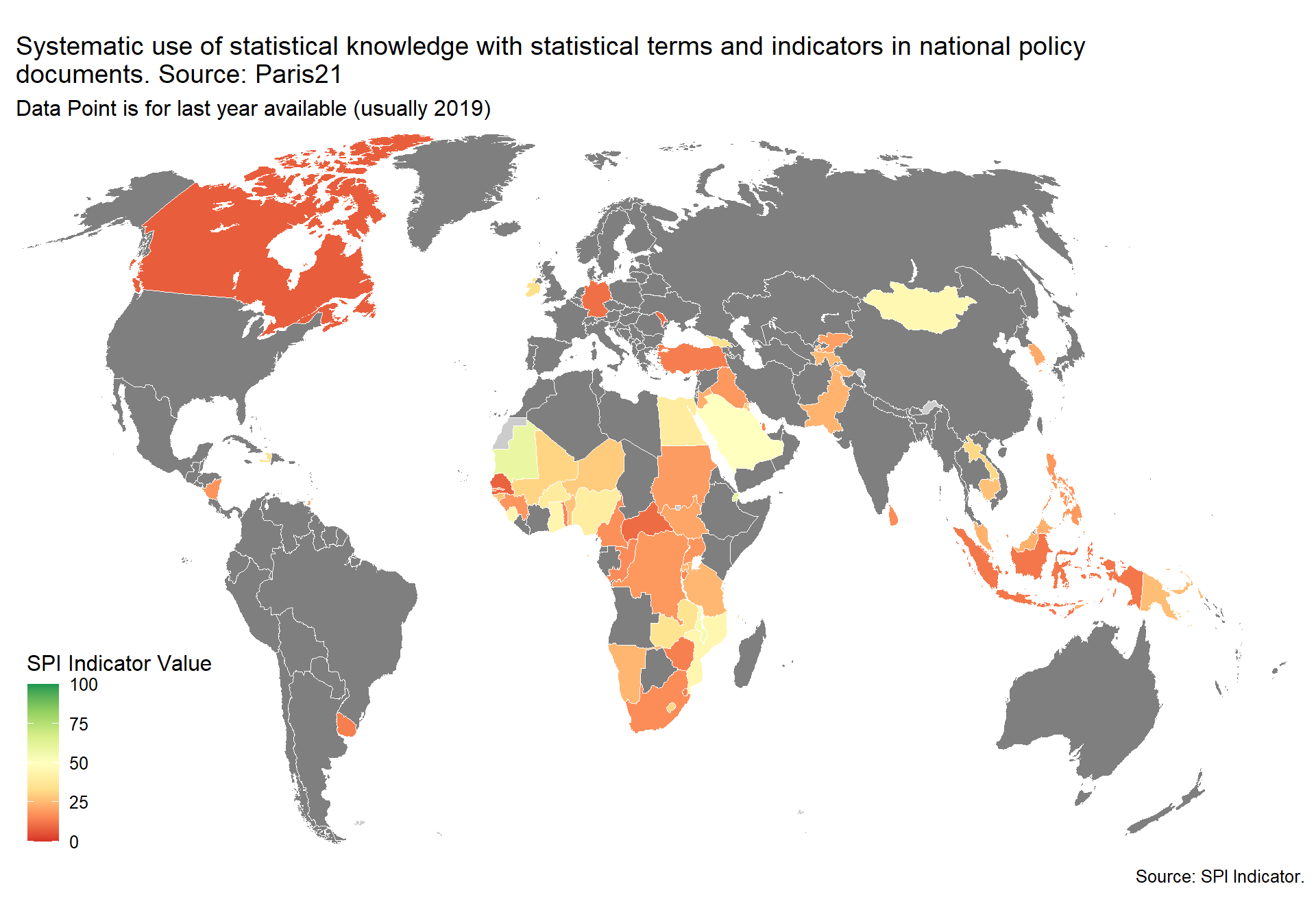
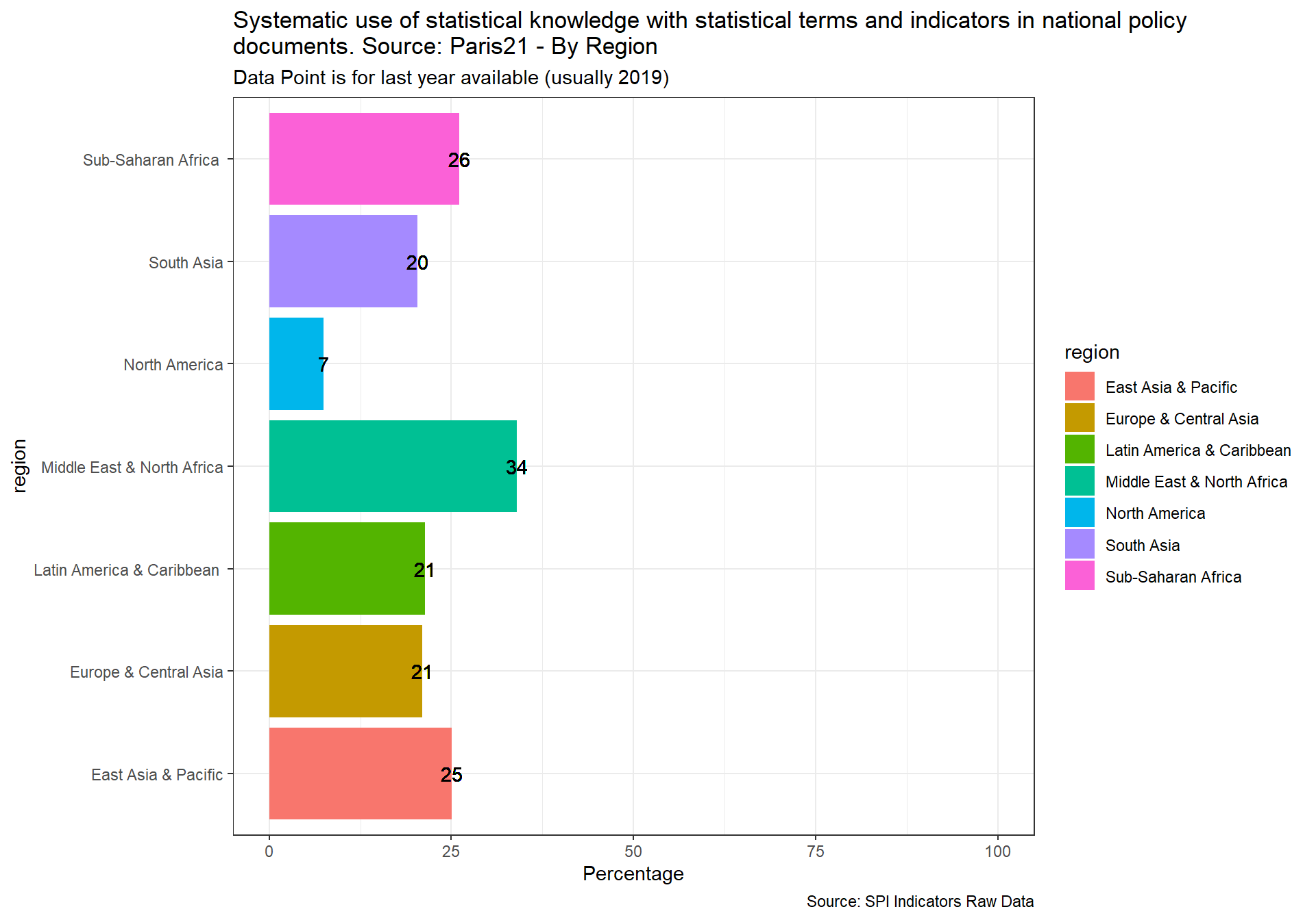
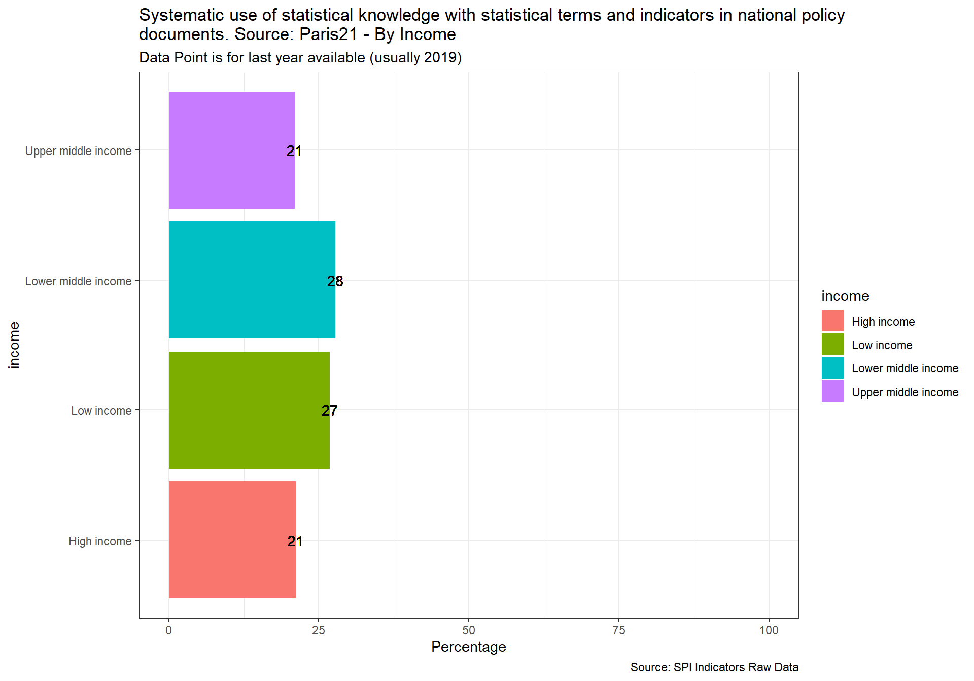
2.5.4 Indicator 5.4: partnerships
Not included because of lack of established methodology or suitable data sources.
2.5.5 Indicator 5.5: finance
Indicator based on SDG indicators (SDG 17.18.3 (national statistical plan that is fully funded and under implementation). This indicator measures whether the national statistical plan under implementation is fully funded. It relates to SDG 17.18.3 and is based on the annual Status Report on National Strategies for the Development of Statistics (NSDS).
Scores is 1 if the country has a national statistical plan that is fully funded and under implementation. Scores of 0 given a score of zero.
The source is Paris 21 and UNSD. Data accessed using UNSD SDG API on 2021-03-24
Source of this data is UNSD and Paris21.
#pull from unsd api
D5.5_DIFI <- un_pull('SG_STT_NSDSFND', '2004', '2019') %>%
  select(iso3c, date,value) %>%
  right_join(spi_df_empty) %>%
  mutate(RAW.D5.5.DIFI=if_else((is.na(value) | value=="NaN"),as.numeric(NA), as.numeric(value)),
         SPI.D5.5.DIFI=if_else((is.na(value) | value=="NaN"),as.numeric(NA), as.numeric(value))) %>%
  select(-value)

## #read in csv file.
## D5.5_DIFI <- read_csv(file = paste(raw_dir, "5.5_DIFI","D5.5_DIFI.csv", sep="/" )) %>%
##   as_tibble(.name_repair = 'universal') %>%
##   transmute(
##     country=Country,
##     date=Year,
##     SPI.5.5.DIFI=Data.Value
##   ) %>%
##     mutate(country=case_when(
##     country=="Bahamas" ~ "Bahamas, The",
##     country=="Bolivia (Plurinational State of)"   ~  "Bolivia"   ,
##     country=="Côte d'Ivoire"  ~  "Cote d'Ivoire"                ,
##     country=="Democratic Republic of the Congo"  ~ "Congo, Dem. Rep."  ,
##     country=="Congo"  ~ "Congo, Rep."        ,
##     country=="Curacao"  ~  "Curacao"       ,
##     country=="Czechia"   ~  "Czech Republic"     ,
##     country=="Egypt"  ~ "Egypt, Arab Rep."        ,
##     country=="Micronesia (Federated States of)"  ~ "Micronesia, Fed. Sts."  ,
##     country=="United Kingdom"   ~  "United Kingdom"    ,
##     country=="Gambia"    ~  "Gambia, The"     ,
##     country=="Iran (Islamic Republic of)"  ~ "Iran, Islamic Rep." ,
##     country=="Kyrgyzstan"   ~  "Kyrgyz Republic"   ,
##     country=="Republic of Korea"   ~ "Korea, Rep."   ,
##     country=="Lao People's Democratic Republic"    ~  "Lao PDR" ,
##     country=="Saint Kitts and Nevis  "   ~ "St. Kitts and Nevis",
##     country=="Saint Lucia"   ~ "St. Lucia",
##     country=="Republic of Moldova"   ~  "Moldova"   ,
##     country=="Democratic People's Republic of Korea"  ~  "Korea, Dem. People’s Rep." ,
##     country=="Slovakia"   ~  "Slovak Republic"             ,
##     country=="United Republic of Tanzania"   ~  "Tanzania" ,
##     country=="United States of America"  ~ "United States"  ,
##     country=="Saint Vincent and the Grenadines" ~ "St. Vincent and the Grenadines" ,
##     country=="Venezuela (Bolivarian Republic of)"  ~  "Venezuela, RB"   ,
##     country=="British Virgin Islands"  ~  "British Virgin Islands" ,
##     country=="Viet Nam"  ~ "Vietnam"        ,
##     country=="Yemen"  ~ "Yemen, Rep.",
##     country=="United Kingdom of Great Britain and Northern Ireland" ~ "United Kingdom",
##     TRUE ~ country
##   )) %>%
##   mutate(RAW.5.5.DIFI=if_else(SPI.5.5.DIFI=='no data',as.character(NA), SPI.5.5.DIFI),
##          SPI.5.5.DIFI=if_else(SPI.5.5.DIFI=='no data',as.numeric(NA), as.numeric(SPI.5.5.DIFI))) %>%
##   right_join(spi_df_empty)

#add to spi databases
spi_df <- spi_df %>%
  left_join(D5.5_DIFI)


D5.5_DIFI_map <- D5.5_DIFI %>%
  filter(!is.na(SPI.D5.5.DIFI))

spi_mapper('D5.5_DIFI_map', 'RAW.D5.5.DIFI', 'Statistical plan fully funded. Source: Paris21')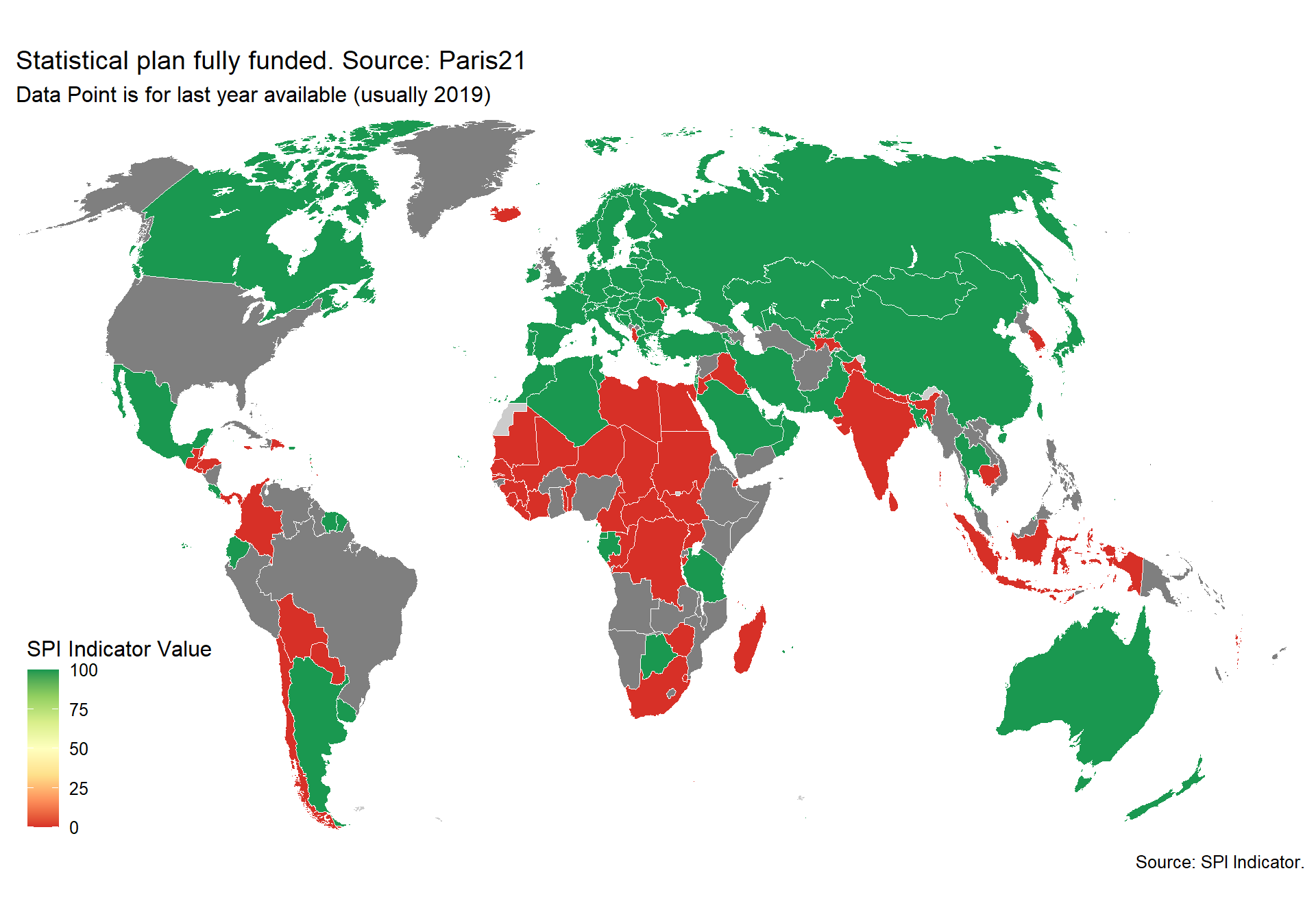
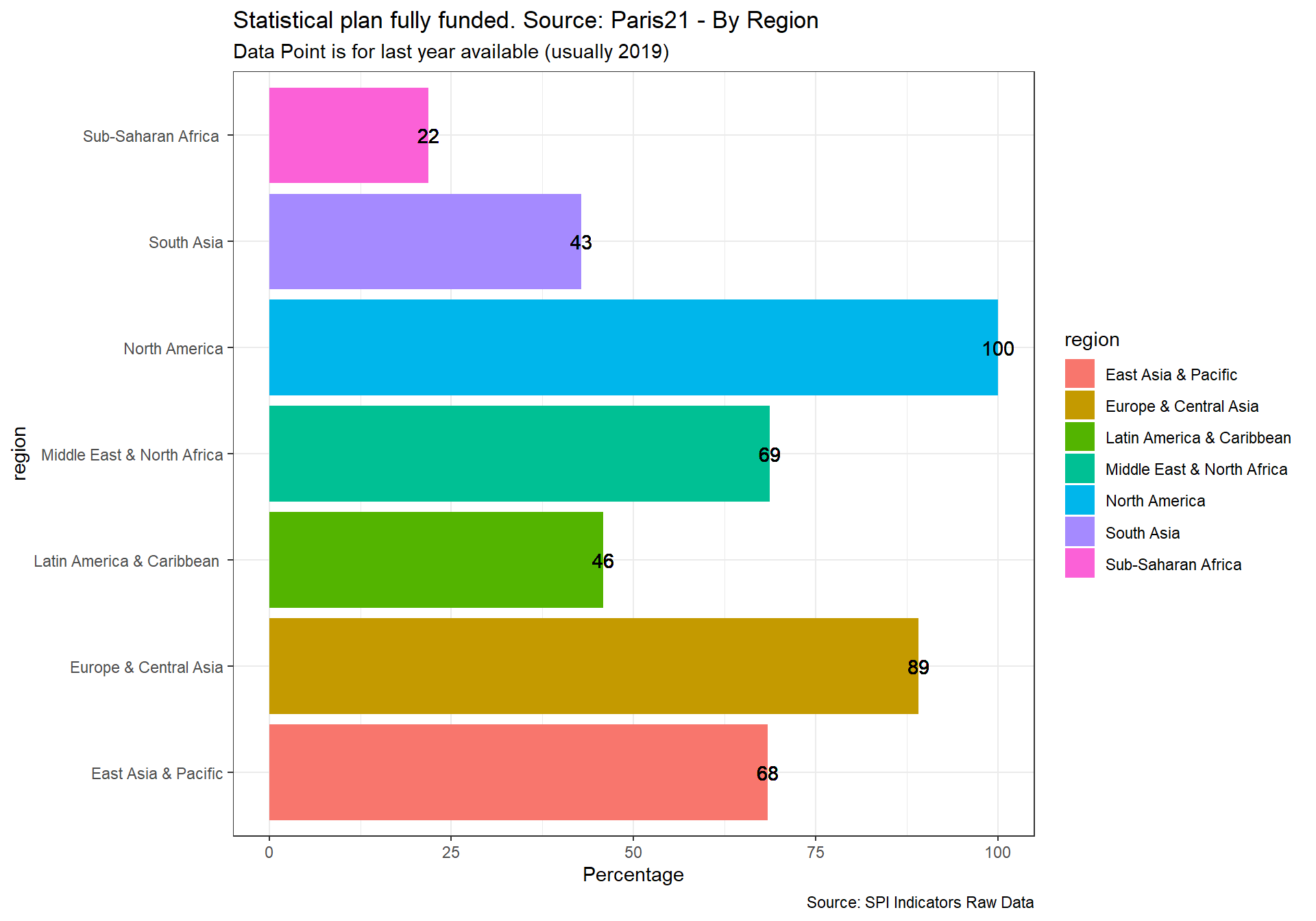
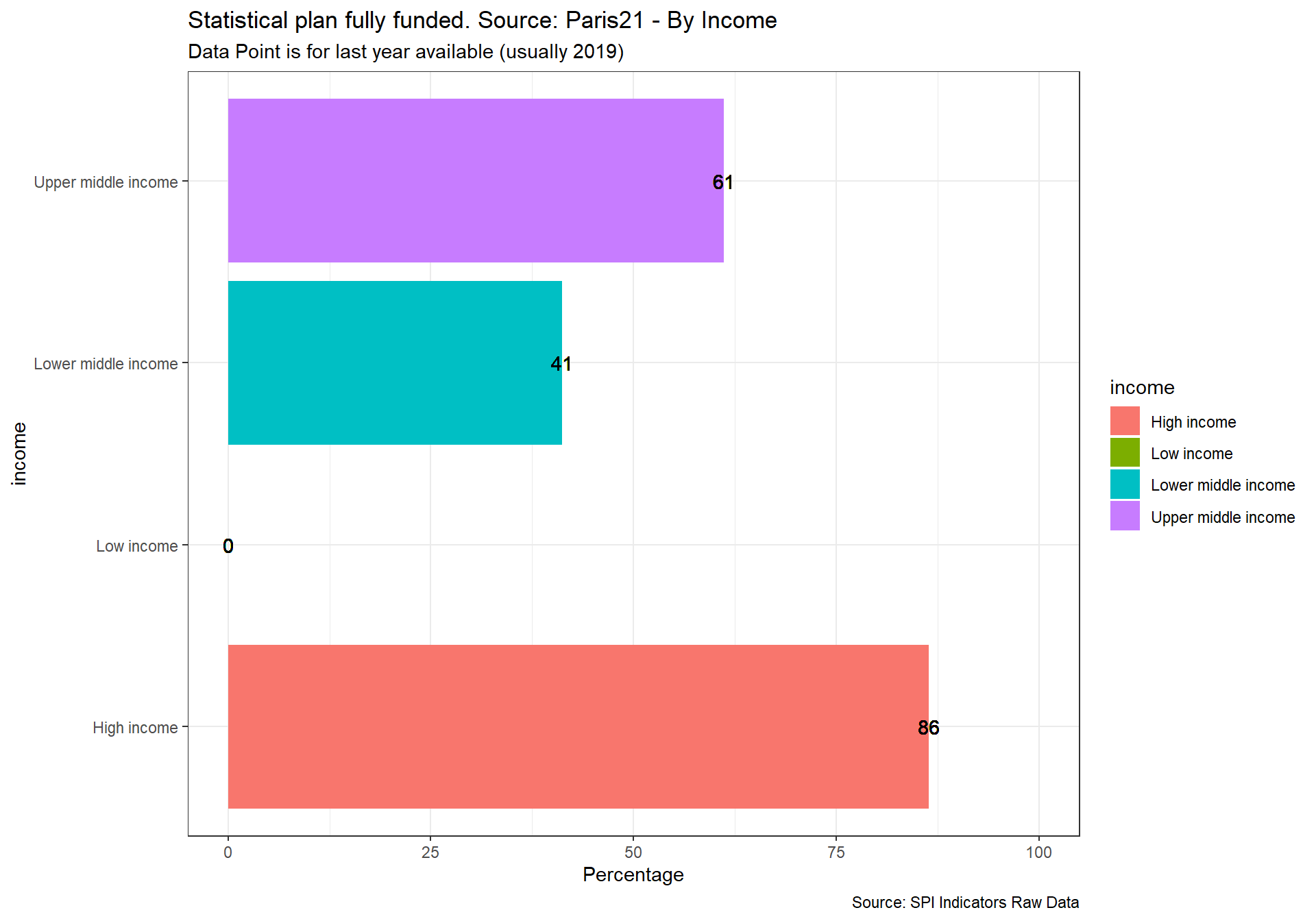
2.6 Final Dataset
Below we will append the data together and save the final files together.
#add in population
pop_df <- wbstats::wb(country="all",
             indicator='SP.POP.TOTL',
             startdate=2004,
             enddate=2019) %>%
  mutate(date=as.numeric(date)) %>%
  mutate(population=value) %>%
  select(country, date, population)

## create final dataset
spi_df_final <- spi_df %>%
  select(country, iso3c, date, starts_with("SPI"), starts_with("RAW")) %>%
  right_join(spi_df_empty) %>%
  left_join(pop_df) %>%
  arrange(-date,country)


####
#lining up data to 2019 and filling in some values for OECD countries.
####
#get a list of oecd countries
oecd_country_query <-  GET(url = "https://api.worldbank.org/v2/country?region=OED&format=json") %>%
  content( as = "text", encoding = "UTF-8") %>%
  jsonlite::fromJSON( flatten = TRUE)

#do some conversion to produce a dataframe
oecd_country_df <- oecd_country_query[[2]] %>%
  as_tibble()

country_mod_list <- oecd_country_df$name  #fill in the missing values for OECDs with 1s because by participating in OECD these countries have this
country_mod_list <- c(country_mod_list, 'Singapore')
spi_df_final <- spi_df_final %>%
  arrange(country, date) %>%
  group_by(country) %>%
  mutate(across(starts_with("SPI"), na.locf, na.rm=FALSE)) %>%
  mutate(across(c("SPI.D1.5.POV",
                  "SPI.D2.1.GDDS",
                  "SPI.D5.1.DILG",
                  "SPI.D5.2.3.CNIN", "SPI.D5.2.5.HOUS", "SPI.D5.2.6.EMPL", "SPI.D5.2.8.FINA",
                  "SPI.D5.2.10.GSBP",
                  "SPI.D5.5.DIFI"),
                ~if_else(( (income=='High income')  & (country %in% country_mod_list)),1,.)                ))
#write to csv
spi_df_final %>%
distinct() %>%
mutate(across(is.list, as.character)) %>%
write_excel_csv( path = paste(output_dir, 'SPI_data.csv', sep="/"))
#label data
#read in metadata
names_df <- data.frame('source_id'=colnames(spi_df_final))
spi_meta <- read_csv(paste(raw_dir, '/metadata/SPI_dimensions_sources.csv', sep="")) %>%
right_join(names_df) %>%
mutate(source_name=if_else(is.na(source_name), paste(source_id), source_name)) %>%
arrange(factor(source_id, levels=colnames(spi_df_final)))
#label data
label(spi_df_final) = as.list(spi_meta$source_name)
#write to stata
spi_df_final %>%
mutate(across(is.list, as.character)) %>%
rename_with(~gsub(".","_",.x, fixed=TRUE)) %>%
select(-lat,-long) %>%
write_dta( path = paste(output_dir, 'SPI_data.dta', sep="/"))