Climate and Agriculture Monitoring in the Pacific Island Countries#
Introduction#
Agriculture is an essential activity for most livelihoods in the Pacific. About 80% of the food consumed in Papua New Guinea (PNG) is produced within the nation, and the largest component of agriculture is subsistence farming. Despite its importance for rural livelihoods, there is a dearth of recent data on agriculture in the public domain.
The populations in the Pacific Island Countries (PIC) are at disproportionately higher risk of adverse consequences from global warming. Current impacts include increasing droughts and water scarcity, coastal flooding and erosion, and changes in rainfall that affect food production (IPCC 2018). Weather conditions and climate variations have profound impacts on agriculture, water resources and on the socioeconomic opportunities and adaptations of the region.
Optical images and climate variables captured by satellites can be a powerful source of information to address data gaps and inform climate assessments. There is a wealth of underutilized satellite data that can be useful to monitor climate events, agricultural productivity, and provide insights for better preparedness and mitigation strategies. Historical and real-time indicators can be a critical input to short and long-term planning, operational decision making, adaptive infrastructure development and the management of climate risks.
The objective of this note is to showcase examples of how public satellite data can inform our understanding of climate risks and agricultural activity in the Pacific region. The examples developed use low-to-medium resolution Earth Observation (EO) data to monitor changes in hydro-meteorological conditions and detect growing seasons. The climate data was collated for the Pacific Observatory and is being made available in tabular and raster formats through the Development Data Catalog.
The note is divided into 5 sections. Sections 1 through 3 address various climate stressors that affect agricultural production in the region. Section 1 presents an overview of climate variability dynamics. Section 2 introduces several climate datasets, including rainfall anomalies and drought indices, and describes use cases where these signals can provide critical insights. Section 3 is dedicated to tropical cyclones. Section 4 showcases how agricultural seasonality parameters can be derived from Vegetation Indices (VIs) produced with optical satellite imagery. The last section introduces a knowledge resource to find data on climate projections.
1. Ocean-Atmosphere Dynamics#
Climate variability directly influences many dimensions of food security, particularly food access and availability. Variation in rainfall is a common element of many natural disasters – droughts, floods, typhoons, and tsunamis – and is influenced by multiple factors.
The main global factor is the El Niño-Southern Oscillation (ENSO, a recurring warm/cool climatic pattern across the Pacific Ocean). Important regional factors include the Madden-Julian Oscillation (intra-seasonal climate disturbance), and fluctuations in sea surface temperature (SST). These are commonly monitored through the West Pacific Gradient (WPG), an index derived from the difference in SST between the NINO4 region and the West Pacific. When the West Pacific is warm during La Niña events, the changes in rainfall across the globe can be extreme. Additional local factors include elevation, island position, the circulation of land and sea breezes, and land cover.
The level of climate risk in the Pacific Island Countries (PICs) can be measured based on the effect of sea surface temperature (ENSO signal) on rainfall variability. Extensive research has examined the impacts of such effects. Loss of food production in Southeast Asia and the Pacific is closely associated with the ENSO phenomena (Naylor et al, 2001, 2007). Anderson specifically indicates ENSO poses risks to crop production in the greater Pacific Basin region (2018).
Inter-annual variability like ENSO also affects fish abundance, distribution, and migration (Lehodey et al, 2006). El Nino years are normally associated with drought years, while La-Niña is often related to wet years which can cause flood hazards in an agricultural context. While in fisheries extended warm pools (East or West) and changes in ocean surface temperature characterize movements of fishes, upwelling of nutrients, and dynamics of prey - predator (due to changing environment).
The following analysis employs a linear regression to examine the correlation between rainfall anomaly and sea surface temperature in each NINO region:
Niño 1 (80°-90°W and 5°-10°S)
Niño 2 (80°-90°W and 0°-5°S)
Niño 3 (90°-150°W and 5°N-5°S)
Niño 4 (150°-160°E and 5°N-5°S)
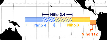
Figure 1. NINO regions. Source: https://www.weather.gov/jetstream/enso
The regression is defined as follows:
Y = aX + b, where: Y = Rainfall anomaly, b = Y intercept, a = Slope and X = SST anomaly
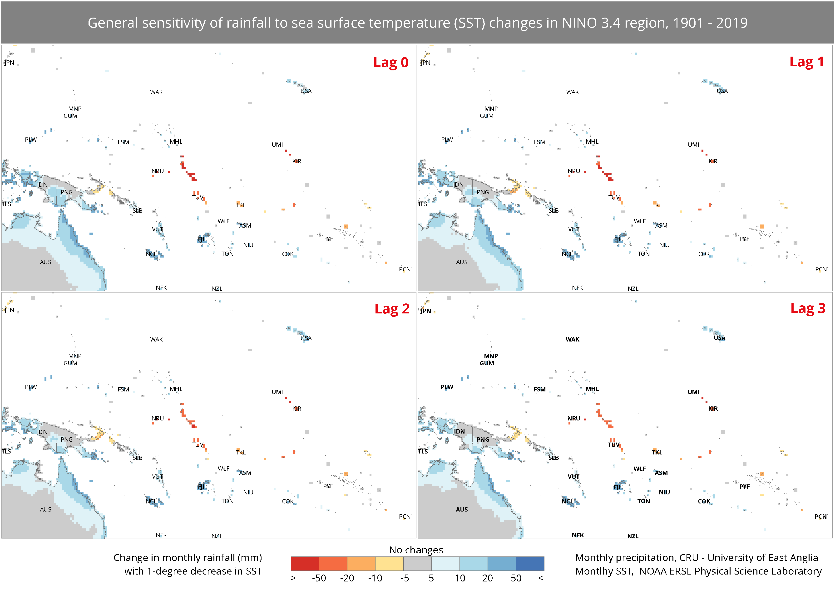
Figure 2. General sensitivity of rainfall to SST changes in NINO3.4 region
The map in Figure 2 demonstrates the change in monthly rainfall associated with a one degree decrease in SST in NINO-3.4 region. Areas highlighted with red (Tuvalu, Kiribati, Nauru, and New Britain and Bougainville Island of PNG) would be severely affected, experiencing 10 to 50 mm below normal rainfall by 1°C change in SST. In contrast, dark blue highlighted areas would experience at least 50 millimeters more of rainfall in the respective month.
ENSO signals used to be the key indicators for agriculture production in some areas. However, negative impacts of the signals to food production have been mitigated with a wide range of adaptations like improvement of irrigation facilities, and innovations in drought and flood tolerant crop varieties. Still, the signals remain critical for hydro-meteorological monitoring and disaster warning.
2. Climate Monitoring Indicators#
This section introduces satellite-derived climate datasets that can be monitored with different temporal resolutions (monthly, daily, and forecast). The variables covered include precipitation, temperature, evapotranspiration, and drought indices. Monitoring these variables in a real-time fashion enables the early detection of water stress in vegetation areas, and helps various actors prepare for climate impacts.
Monthly and Seasonal: SPEI#
The Standardized Precipitation-Evapotranspiration Index (SPEI) is an established indicator to detect, monitor, and analyze droughts. The SPEI considers how various climate variables (precipitation, evapotranspiration, temperature) relate to normal conditions and can be calculated according to different temporal scales. The multi-scalar character of this indicator makes it a suitable proxy to identify dry and wet conditions related to soil moisture, which can have significant impacts on agriculture.
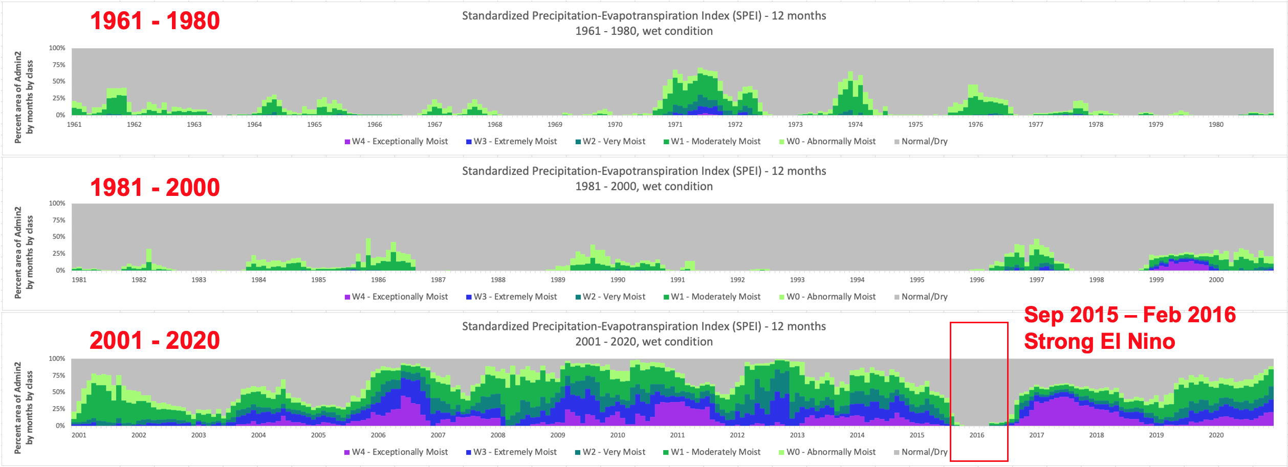
Figure 3. Wet condition in PNG, 1961-2020 (Terra Climate)
Figures 3 shows the share of districts that experienced high levels of SPEI (signaling wet conditions) by month. In December 2020, close to 70% of districts in PNG experienced wet conditions, 20% were exceptionally wet, and only about 10% experienced normal conditions. Showing the inverse of Figure 3, Figure 4 indicates months with dryer than usual climate. PNG has been relatively wet in the last 20 years, although the ENSO signal drove a significant dry period during 2015-2016 (strong El Nino).
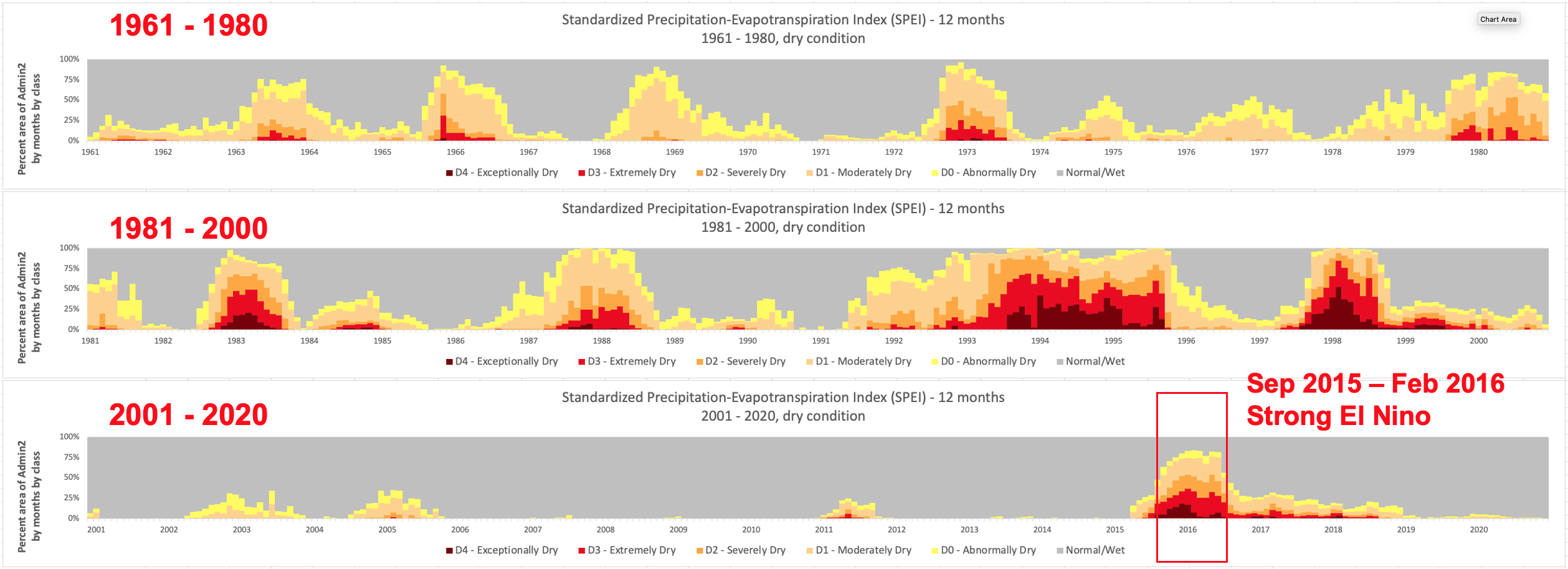
Figure 4. Dry condition
Monthly SPEI data can provide valuable lead time to identify the slow onset of cumulative climate impacts. The data can help discern how the dry or wet situation is evolving month-by-month, year-by-year. The maps below show the spatial disaggregation in the SPEI data, highlighting the contrast from two time periods with drastically different trends: December 2015 (Strong El Nino) and December 2020 (Moderate La Nina).
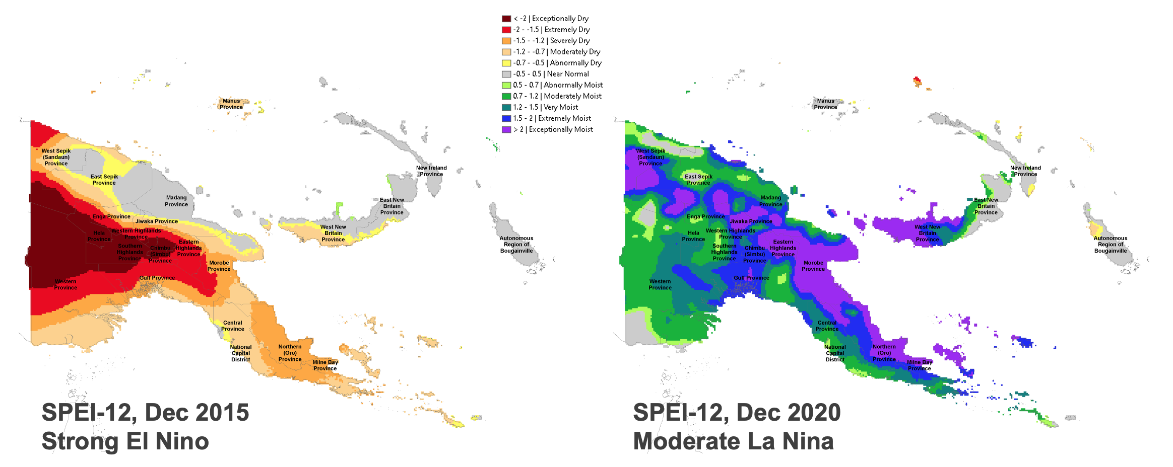
Figure 5. SPEI 12-months
Long-term historical information is a key resource to understand past climate events, identify variable impacts across regions, and study how water demand continues to be affected by increasing temperatures.
As alternative to the SPEI, we may also consider a newly-developed NOAA tool – EDDI, or the Evaporative Demand Drought Index – works a little differently from PDSI and other drought indices (such as SPI, NLDAS, and the Climate Prediction Center’s modeled soil moisture products & remotely sensed actual evapotranspiration), to have a more comprehensive understanding of drought and how it is analyzed.
EDDI was developed exclusively to monitor atmospheric evaporative demand (E0), also described as atmospheric “thirst.” Over shorter time frames of weeks and months, EDDI provides early warning for rapidly evolving flash droughts and indicates the persistence of ongoing drought. The archive of the global Evaporative Demand Drought Index (EDDI; Hobbins et al. 2016, McEvoy et al. 2016) service is freely available to all from NOAA website.
Daily#
Daily estimates of extreme rainfall are available based on satellite microwave precipitation estimates. The following section demonstrates how daily weather data can be utilized to inform early warning systems and disaster response policies.
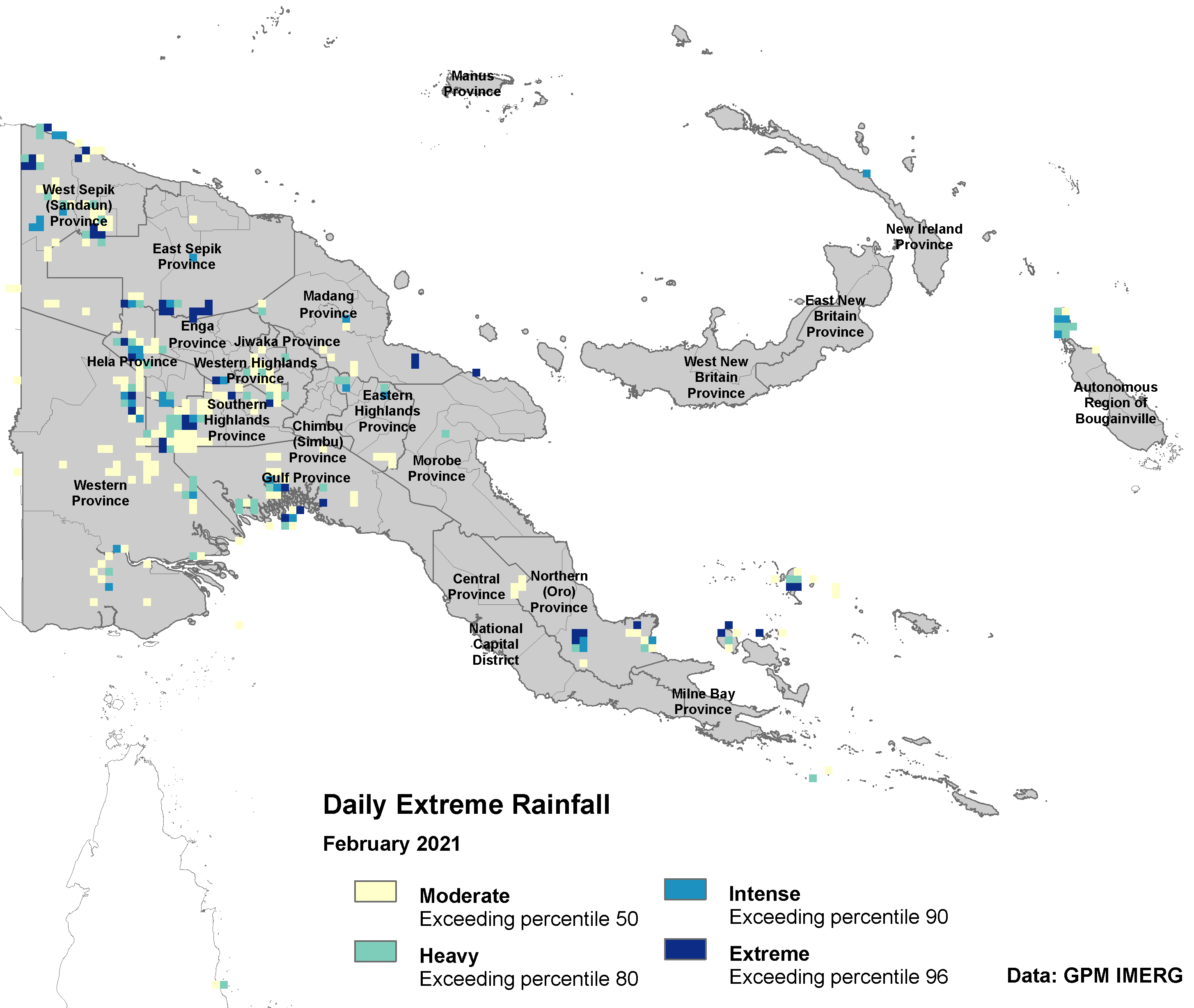
Figure 6. Extreme rainfall
Daily rainfall data can inform policy through various mechanisms:
Input to early warning systems and trigger anticipatory actions.
Will it cause a landslide?
Which roads will be affected?
How many populations and cropland will be affected?
Which area is in early planting and will be damaged?
Another multi-temporal indicator of meteorological conditions is maximum consecutive dry days (CDD). This index captures the cumulative effect of consecutive days without precipitation (days with less than 1 mm of rain). CDD can be updated on daily basis and serve as an effective measure of seasonal droughts.
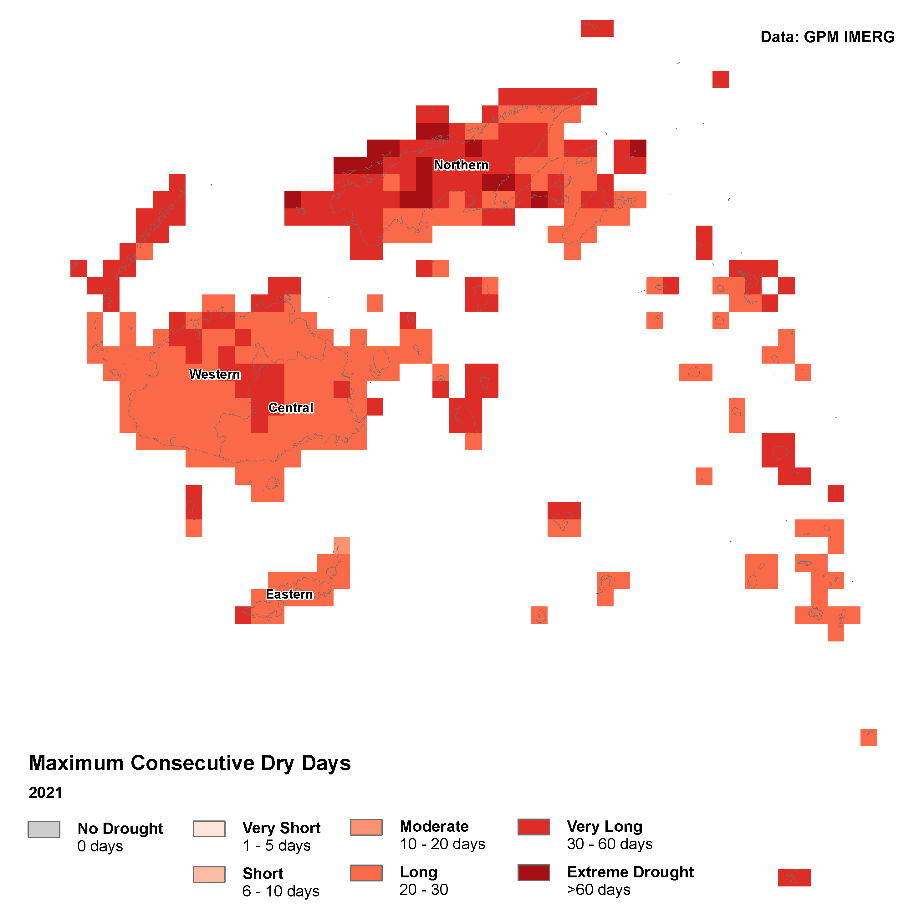
Figure 7. Maximum consecutive dry days in 2021
Weather datasets uncertainty and issue of scale#
All climate monitoring products mentioned above are based on satellite precipitation estimates or modeled products. The accuracy may vary according to landscape characteristics, modeling method, number of stations available for model inputs, and other aspects relevant to data granularity.
Assessment of accuracy for the region, might be useful, either by comparing to ground records at weather stations or across weather data products of similar resolution (Terra Climate, CHIRPS, SM2RAIN-ASCAT, IMERG, etc.). For the case of the Pacific, availability of weather stations across the region is challenging. As one alternative to observation data, we could use CPC Global Unified Gauge-Based Analysis of Daily Precipitation (GUGBADP) from the NOAA Physical Science Laboratory.
Bias correction#
Bias correction is the most common method to increase the quality of secondary products such as satellite-based precipitation data. This method is also widely used to correct the general circulation model (GCM) on both long-range climate forecast and climate projection. There are many methods that can be used to carry out bias correction, such as the daily data is simply shifted by the mean bias in the reference period (Hawkins et al., 2013) or possible to apply a more general form of this bias-correction method that corrects not only the mean values but also the temporal variability of the model output in accordance with the observations (Hawkins et al., 2013; Ho et al., 2012. Another method would be the Change Factor (CF) approach, where the value is subtracted from the future simulated values, resulting in “climate anomalies” which are then added to the present-day observational dataset (Tabor, K. and Williams, J.W., 2010).
The above-mentioned methods work well for more non-stochastic variable (i.e., temperature), while for more stochastic variables (e.g., precipitation and solar radiation), we need to ensure realistic daily and interannual variability. Empirical Quantile Mapping (EQM) is one of the most widely used and common techniques for this purpose. Like many other bias correction methods, EQM is well-known amongst climate scientists and practitioners in modeling, especially those specialized in climate projection. EQM offers simple yet rather powerful technique (Wood, et al., 2002), and the result is rather satisfying in increasing precipitation related GCM (Enayati, et al., 2020; Themeßl, et al., 2012; Gudmundsson, et al., 2012; Sachindra, et al., 2014). EQM uses probability density function (PDF) and cumulative distribution function (CDF) to correct raw data i.e., GCM models, satellite-based products etc. EQM will change the corrected distribution dataset to match the in-situ observation.
Improved on near real-time daily Rainfall Estimate (RFE) availability#
The Pacific region spans a large area, with land masses of different sizes and terrains. The reliance on public use datasets is important for sustainability of the initiative but limits the granularity of data for monitoring. For daily monitoring, the analysis relies on IMERG data which available in 0.1 degree and this is the best publicly available near real-time data for precipitation which are useful for consecutive dry days and extreme rainfall monitoring, but the spatial resolution is to coarse for the Pacific Islands which consist of many small islands.
There is a new product which will release in near future from Climate Hazard Center - UCSB named Climate Hazards center IMErg with Stations (CHIMES), which enhances the IMERG Late Run product using an updated Climate Hazards Center’s (CHC) high-resolution climatology (CHPclim) and low-latency rain-gauge observations, resulting in a product that is similar to IMERGfinal, but with a lower latency (Funk et al. 2022).
Further analysis on comparing the outputs from higher resolution sources for both vegetation indices (Sentinel) and precipitation (CHIMES) would help to illustrate impact on analysis of using data at finer spatial resolution.
3. Cyclones#
Cyclone patterns are important to track in the Pacific as they can indicate which areas are more vulnerable and likely to suffer loss of agricultural production due to extreme rainfall. Traditionally, areas of tropical cyclone (TC) formation are divided into seven basins. Impacts of cyclones typically are related to the high amount of rainfall and strong wind they bring. Recent tropical cyclone Harold in 2020 flashed large area of crops in Vanuatu and Fiji. There are also times when the damage is higher than the country’s GDP, such as Cyclone Ofa and Val that hit Samoa in 1990/1991.
Western Pacific Ocean#
The West Pacific Ocean is the most active basin on the planet, accounting for one-third of all tropical cyclone activity. Annually, an average of 25.7 cyclones in the basin acquire tropical storm strength, and an average of 16 typhoons per year were recorded during 1968 to 1989. The basin sees activity year-round, but cyclone activity is at its minimum in February/March.
Manganello, et.al. ((2013)[https://doi.org/10.1175/JCLID-13-00678.1]) studied the 16-km ECMWF Integrated Forecast System (IFS) also projects about a 50% increase in the power dissipation index, mainly due to significant increases in the frequency of the more intense storms. The development rate and the peak intensities of these storms increase in a future climate, which is consistent with their tendency to develop more to the south. Other major changes in future TC activities over the West Pacific are associated with the Accumulated Cyclone Energy (ACE) and intensity. The future ACE of total TCs shows a significant increase because individual TCs have a longer lifetime and higher maximum wind speed compared to those in the historical run. Although the change in the total number of TCs is not very large, the regions affected by the TCs are changed as TC intensity increases, especially in midlatitudes according to recent study from Lee, et.al. (2019[https://doi.org/10.1175/JCLI-D-18-0575.1]).
South Pacific Ocean#
Tropical Cyclones that develop within the South Pacific basin generally affect countries to the west of the international dateline, though during years of the warm phase of ENSO cyclones have been known to develop to the east near French Polynesia. On average, the basin sees nine tropical cyclones annually with about half of them becoming severe tropical cyclones.
During December to May cyclone events occur mostly in the South Pacific Ocean, whereas from June to December most cyclone events happen in West Pacific Ocean.
Zhang and Wang (2017[https://doi.org/10.1175/JCLI-D-16-0597.1]) identified the 20-yr mean TC genesis frequency over the South Pacific consistently decreased. The future change in TC genesis frequency in the peak season is not significant in the West Pacific, but it decreased significantly in the peak season in the South Pacific. The frequency of TC occurrence over the South Pacific decreases at all intensities in the future runs mostly due to the large reduction of TC genesis frequency under warmer climate conditions.
It is important to note that these studies are based on the assumption of a particular scenario of greenhouse gas emissions and climate change, and the actual future development might vary. Additionally, tropical cyclone forecasting, and projection is still a complex and challenging task, and further research is needed to improve the understanding and predictability of tropical cyclones in the Western Pacific Ocean and South Pacific Ocean.
Agriculture Monitoring#
Climate and vegetation data sourced from satellites are widely used for agricultural monitoring, especially in the planting and growing season. Agricultural monitoring with remote sensing is often conducted with medium-low resolution imagery because public satellites provide long-term coverage and stable revisit rates. This data can provide useful information for:
Providing early warning before climate shocks threaten food security.
Contextual analysis needed to plan interventions. For example, market operations when crop scarcity occurs.
Availability of cropland area for subsequent planting after losses due to conflict or disasters.
Whether food is produced by households or bought from local markets, for domestic consumption or commercial purpose, earth observation can be a powerful tool to provide information on the status of cultivation and harvested areas.
Agriculture monitoring outputs are promising for remote sensing-based yield analysis. However, obtaining local data of crop extent mass remains a challenge. Crop type and yield mapping for ground truthing are not widely available. Though, there are options from crop models e.g., SCYM, WRSI, etc. for major crops. This should be noted for further development and analysis, for example localized extreme events on crop specific yield. At this point, the analysis is also limited to seasonal crops due to difficulty to capture the dynamics of perennial crops within a year and lack of crop extent map.
Remote sensing data requirements for vegetation monitoring#
Operational data production
Data needs to be available on a routinely basis, ideally with a set time interval.
Definition of historical conditions
Historical averages are useful to then calculate anomalies, deviations from normal conditions, percentage change, or ranking maps. These statistics are critical to explain how current conditions compare to the historical conditions for a specific location and time during the year. They also enable the differentiation of moderate, severe, and extreme drought events.
Vegetation Indices#
The Enhanced Vegetation Index (EVI) is an optimized index designed to enhance the vegetation signal detected from optical images. The index attempts to improve sensitivity in high biomass regions, de-couple the canopy background signal, and reduce atmospheric influences in the vegetation signal.
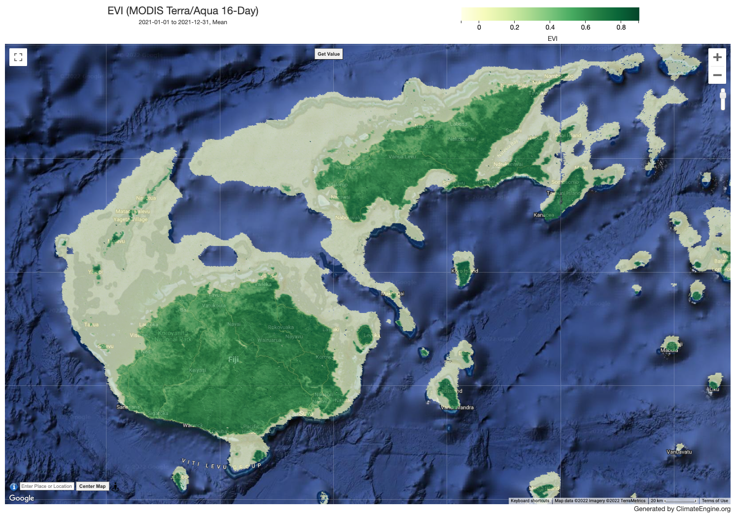
Figure 8. EVI index in Fiji, 2021 (Data source: MODIS, retrieved from Climate Engine).
While the Normalized Difference Vegetation Index (NDVI) is chlorophyll sensitive, the EVI is more responsive to canopy structural variations, including leaf area index (LAI), canopy type, plant physiognomy, and canopy architecture.
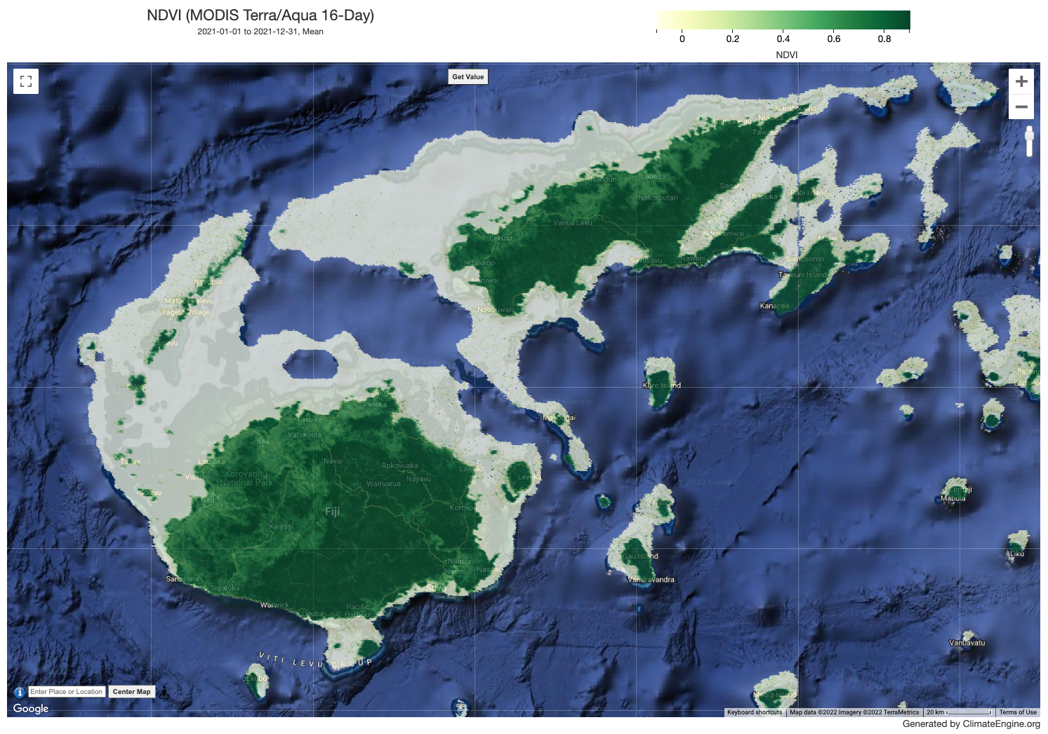
Figure 9. NDVI index in Fiji, 2021 (Data source: MODIS, retrieved from Climate Engine).
Methodology#
A working example to detect seasonality parameters in PNG has been developed based on areas where the majority of cropland is paddy. This approach requires a crop type mask and moderate resolution time series Vegetation Indices (VI). In this example, we use data from the MODIS Terra Vegetation Indices (MOD13Q1), available at 250m spatial resolution and temporal intervals of 16 days.
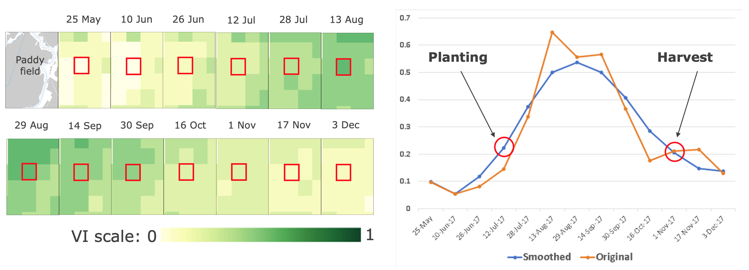
Figure 10. Growing season detection on a paddy field
State of planting and harvesting estimates are determined by importing Vegetation Indices (VI) data into TIMESAT – an open-source program to analyze time-series satellite sensor data. TIMESAT conducts pixel-by-pixel classification of satellite images to determine whether planting has started or not. This process is followed for all areas over multiple years to evaluate current planting vis-à-vis historical values from 2003 - 2021 (in this case with MODIS EVI data).
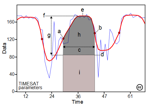
Figure 11. TIMESAT Parameters
The main seasonality parameters generated in TIMESAT are (a) beginning of season, (b) end of season, (c) length of season, (d) base value, (e) time of middle of season, (f) maximum value, (g) amplitude, (h) small integrated value, (h+i) large integrated value. The blue line in Figure 11 shows the raw EVI time series, while the red line shows the EVI values after applying a Savitsky-Golay smoothing algorithm. The phenological parameters detected describe key aspects of the timing of agricultural production and are closely related to the amount of available biomass.
Phenological events are sensitive to climate variation. Therefore, phenology data provide important baseline information to assess ecological trends and identify climate change impacts. Comparing current VI values with the long-term averages, and with minimum and maximum values, helps to better understand the performance of the vegetative season and its expected productivity.
Growing Season#
Decision makers can plan for better outcomes by knowing when the onset of planting happened, or the estimated harvest time.
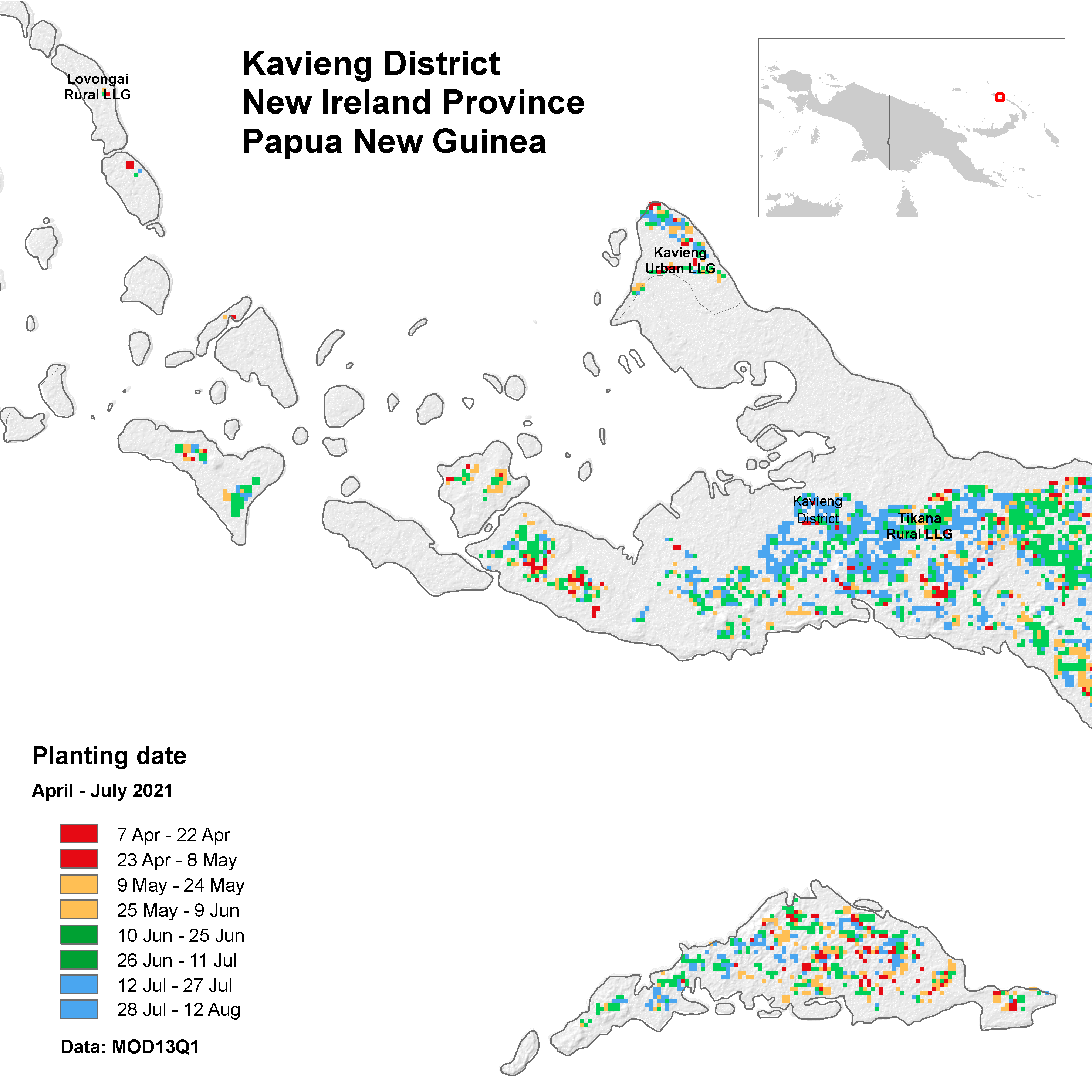
Figure 12. Map of planting date in Kavieng District, PNG. Produced with MODIS data using Timesat software.
The map in Figure 12 shows the start of the season, or planting date, for crop areas across Kavieng District. This map provides an important starting point for continuous monitoring of the crop planting status. Continuous monitoring could inform the following assessments:
How many districts are behind in planting? If there is a delay in some districts, and is planting acceleration necessary?
How many hectares are available for the next season?
Is the current harvest enough for domestic consumption?
Decision makers also need phonological data to decide on resource allocation issues or policy design:
Planting potential for the next months: assigning the distribution of agricultural inputs.
Mobilization of extension workers to monitor and implement mitigation strategies: adjustment of irrigation system in anticipation of drought or flood, pest control of infestation/disease to avoid crop failure, reservoir readiness for planting season.
Preparation of policy recommendations: assess ongoing situation, harvest estimate, price protection.
This information is necessary for both policy makers, farmers, and other agricultural actors (cooperatives, rural businesses). Negative consequences can be anticipated months ahead and resources can be prioritized on areas with higher risk or greater potential.
Limitations and Assumptions#
Obtaining high-quality VI data for all timesteps is challenging due to frequent interruptions caused by clouds. Figure 13 shows a high number of timesteps in 2020 for which the Sentinel-2 satellite captured a cloudy image for a selected crop area. Vegetation Indices based on Synthetic Aperture Radar (SAR) are a good alternative as they can see through clouds and should be explored further in the Pacific context.
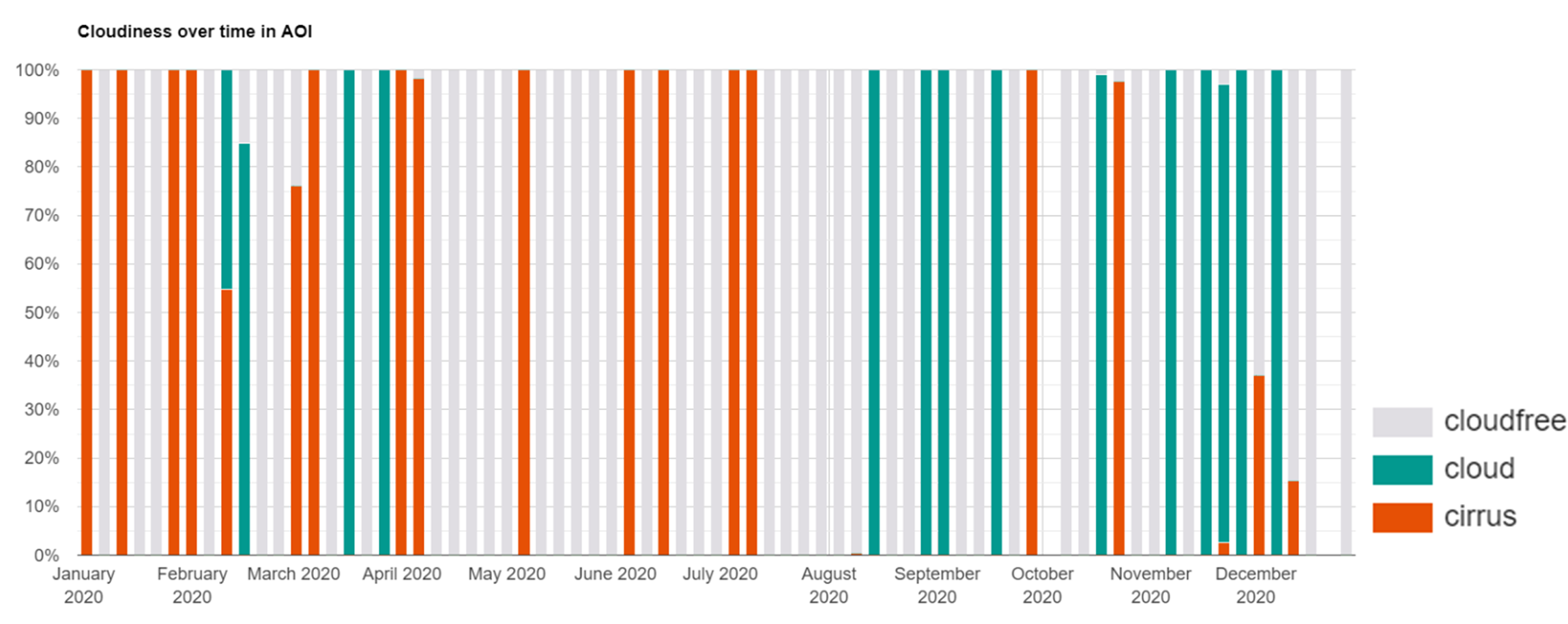
Figure 13. Sentinel-2 data quality for a selected crop area in the Eastern Highlands, PNG
Other data quality issues with optical imagery include snow/ice, aerosol quantity, and shadows. Due to these factors, the quality of MODIS or Sentinel-2 data varies per year, making it difficult to compare VIs and estimated cultivated area. This analysis was based on publicly available MODIS data and a global cropland extent map from the Global Food Security-Support Analysis Data (GFSAD). Because this map only provides a binary indication of where crops are, the seasonal parameters presented are for general cropland. Further research and resources need to be devoted to produce region-specific datasets that differentiate specific types of crops.
Forecasts and Future Projections#
Forecast#
In general, short-term weather forecasts (for the next few days) tend to be more accurate than longer-term climate forecasts (for the next few months or years). This is because weather patterns can change rapidly and unpredictably, whereas climate patterns tend to be more stable and predictable.
Forecast information can be acted upon as soon as it is available, but the level of confidence in the forecast will depend on the time frame being considered. For example, a forecast for the next 24 hours will have a higher level of confidence than a forecast for the next 7 days. It is always important to consider the source of the forecast and the level of confidence in the information before taking any actions.
Sub-seasonal and seasonal forecasts of precipitation and temperature are available via the International Research Institute (IRI) of Columbia University . The forecasts provide relevant information for key events, such as the timing of the onset of the rainy season, important for agriculture, or the risk of extreme rainfall events or heat waves, critical for public safety. In Figure 14 and 15, shades of brown indicate a forecast of drier conditions, whereas shades of blue indicate a forecast of wetter conditions.
1. Sub-seasonal Forecast: Optimum planting and harvest potential#
Sub-seasonal forecasts predict key variables (temperature or precipitation) on a weekly basis up to one month ahead. Historical records of planting in combination with these forecasts are helpful to draw a recommendation on optimal planting dates. Weather forecasts released during the 2nd or 3rd planting season enable actors to plan for optimum yield, meaning that they can identify which type of crops will grow best given the forecasted precipitation level. Similarly, the forecasts can identify which areas can grow secondary crops and inform decisions over how to distribute seeds.
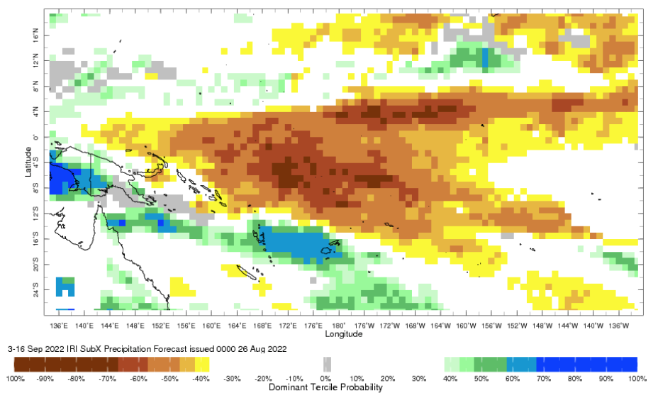
Figure 14. Sub-seasonal Forecast Precipitation. Source: IRI
2. Seasonal Forecast: Opportunities during climate extreme events#
Seasonal forecasts provide longer time-intervals and are usually available up to 7 months in advance. Sub-seasonal forecasts are more accurate than seasonal forecasts as they predict less far into the future. Seasonal forecasts are necessary for optimizing harvest in the long-term. If a planted area is damaged by a flood or drought event, replantation programs can be designed considering long-term forecasts. Replantation programs can be initiated if long-term rainfall forecasts are favorable.
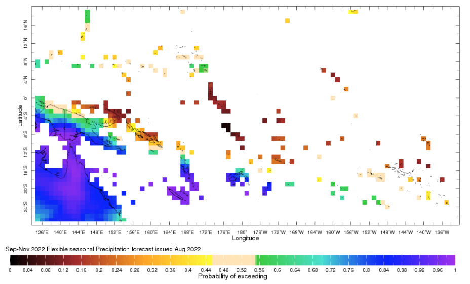
Figure 15. Seasonal Forecast Precipitation. Source: IRI
Future Projections#
Future changes in climate will have significant impacts in agriculture. In PNG, changes in precipitation, temperature, and the frequency of severely warm or cold days will be a determining factor of future crop yield. Climate projections can be used to approximate the magnitude of these impacts.
The WBG Climate Change Knowledge Portal CCKP provide projections for annual number of days with heat index greater than 35°C, precipitation anomalies, and maximum temperature anomalies. This data can serve as the basis for projecting changes in crop yield.
For example, Elisabeth Vogel et al. (2019) identified sensitivity of maize, soybeans, spring wheat, and rice to warm day frequency and cold night frequency. Easterling, W. E. et al. (2007) studied cereals, wheat, and rice sensitivity to 1°C increase of temperature in a different latitude. Changes in short-term temperature extremes can also be critical if they coincide with key stages of development. Wheeler et al. (2000) identified only a few days of extreme temperature (greater that 32°C) at the flowering stage of many crops can drastically reduce yield.
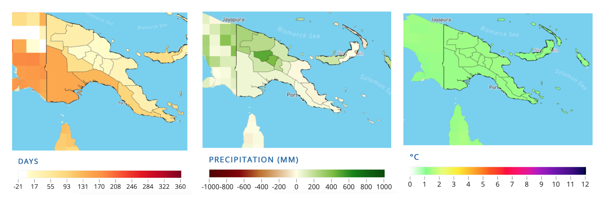
Figure 16. PNG Projections: Annual number of days with heat index > 35oC, Anomaly of precipitation, and Anomaly of maximum temperature in 2040 – 2059..[^1]
The maps are based on Shared Socioeconomic Pathways (SSPs) Scenario 8.5 (worst scenario) for the period 2040 - 2059. Reference period: 1995 – 2014. This type of data is critical for the design of adaptation measures and long-term agriculture development plans.
Map Disclaimer
Country borders or names do not necessarily reflect the World Bank Group’s official position. This map is for illustrative purposes and does not imply the expression of any opinion on the part of the World Bank, concerning the legal status of any country or territory or concerning the delimitation of frontiers or boundaries.
Acknowledgement
This feasibility note was written by Benny Istanto, with additional support from Andres Chamorro. The team gratefully acknowledges the Australian Department of Foreign Affairs and Trade for funding the analysis through the Pacific Observatory. The team is thankful for the guidance from Utz Pape and David Gould (Task Leaders for the Pacific Observatory), and to Siobhan Murray and Alwin Hopf for their support in reviewing this work.