2. Gathering and Preparing the Data Set

Gathering and preparing data is a process that requires great care. Prior to documenting a dataset, it is important to ensure that you are working with the most appropriate version of all the concerned data files. If the dataset is meant for public release, one should work with the final, edited, anonymous version of the dataset. If the dataset is being documented for archiving and internal use only, one may include the raw data as well as the final, fully edited files. If you are working with administrative data, more information on documentation of administrative data is provided in the annex. The Metadata Editor provides you with the possibility of documenting the specificity of each version of the dataset.

Much of the quality of the output generated by the Editor will depend upon the prior preparatory work. Although you can make changes to the data from the Metadata Editor, it is highly recommended that the necessary checks and changes be made in advance using a statistical package and a script. This ensures accurate and replicable results.

This section describes the various checks and balances involved in the data preparation process, such as: making a diagnostic on the structure of your data, cleaning it and identifying the various variables at the outset. Listed below are some common data problems that users encounter:

• Absence of variables that uniquely identify each record of the dataset
• Duplicate observations
• Errors from merging multiple datasets
• Encountering incomplete data when comparing the content of the data files with the the source documentation, data collection instruments, data specifications, or system design documents
• Unlabelled data
• Variables with missing values
• Unnecessary or temporary variables in the data files
• Data with sensitive information or direct identifiers

Some practical examples using a statistical package are provided in Section A: Data Validations in Stata.

Note: If you are working in a data archive, be careful not to overwrite your original variables. Since managing databases involves several data-checking procedures, archive a new version in addition to the original. Work on this new version, leaving the original data files untouched.

The following procedures are recommended for preparing your dataset(s):

2.1. Data Files Should Be Organized in a Hierarchical Format

Look at your data and visualize it to understand its structure. It is preferable to organize your files in a hierarchical format instead of a flat format. In a hierarchical format, columns contain specific information about all possible units of analysis and rows form the individual observations (households, establishments, products, communities/countries, or any combination of those). Hierarchical files are easier to analyse, as they contain fewer columns that store the same information and are more compact. A flat format contains multiple columns with information on only one specific unit of analysis, so the information becomes redundant. For example, the information provided in one column is about the household head, and the row provides information on the child in the household.

Table 1. Flat Format

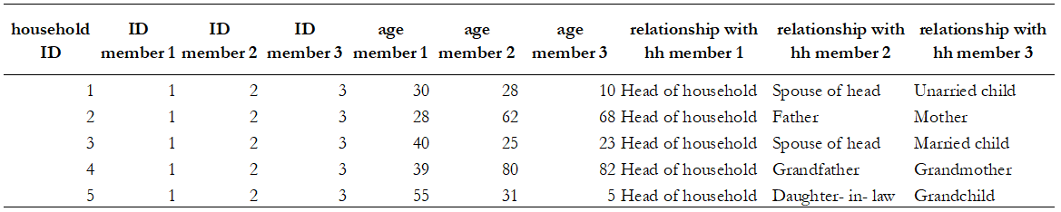
Table 2. Hierarchical Format

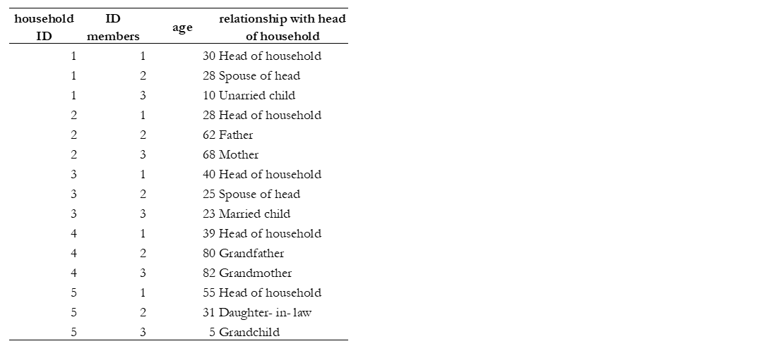
Tables 1 and 2 illustrate the two data structures. They contain the same information about six people on age and their relationship with the head of the household. The flat dataset (Table 1) stores the information on each family member in a new column. Note that for every additional member or characteristic, the dataset gets flatter and wider. The hierarchical dataset (see Table 2) has one observation and one row per person. Each variable contains a value that measures the same attribute across people and each record contains all values measured on the same person across variables. For every additional member characteristic, the dataset maintains the same number of columns, gains additional rows and gets longer and less flat compared to Table 1. The first two columns of this dataset have a hierarchical structure, where the ID member column is nested inside the ID household column.

Hierarchical files are easier to manage. Suppose in this example that there were many characteristics measured for everyone, the hierarchical structure would be a more convenient format because for each new characteristic, the dataset creates only one additional column, whereas, in the flat structure, it would create as many columns as there are people in the data with such characteristics.

Datasets With Multiple Units of Analysis Should Be Stored in Different Data Files

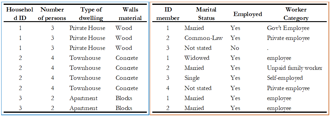
It is recommended that you store your data in different files when you have multiple observational units. For example, Table 3 shows a dataset that has both household-level data (columns on the type of dwelling and walls material) and individual-level data (columns on the marital status, work status, and worker category). Note that storing both levels of information in one dataset will result in a repetition of household characteristics for each household member. In Table 3, the information about the columns 'type of dwelling' and 'wall material' is repeated for everyone. Sometimes, this duplication is inefficient, and it is easier to have the dataset broken down by observational unit, into multiple files. In this example, it would be simpler to create two files: one for the household characteristics and another for the individual characteristics. The two files can be connected through a unique identifier, which in this case will be the household ID and member ID. We discuss the need for this unique identifier further on in this text as well.

Table 3. Single data set with more than one observational unit

Columns in a Dataset Should Represent Variables, Not Values

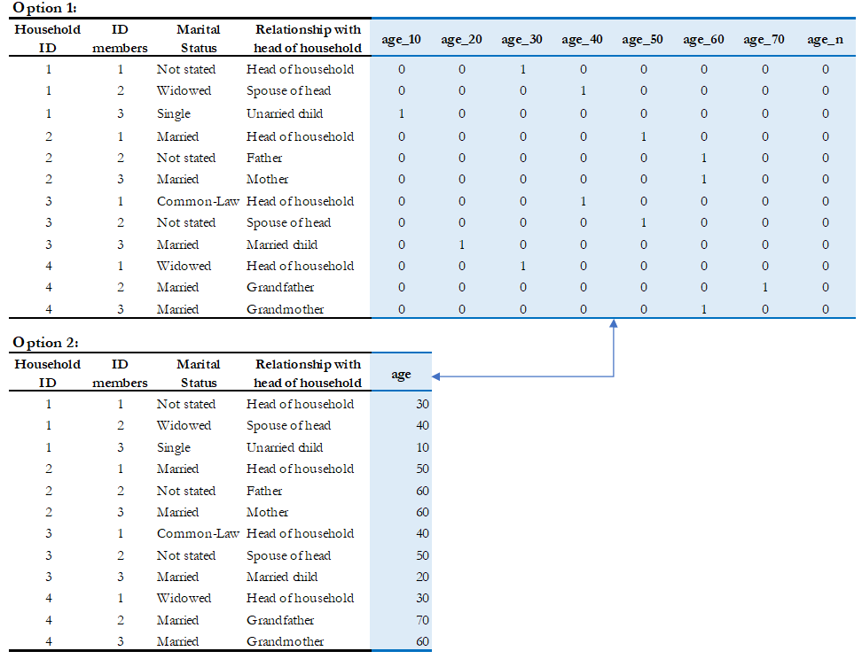
It is recommended that columns represent variables (e.g., sex, age, marital status) and rows represent observations (e.g., individuals, households, firms, products and so forth). In some datasets, columns instead of describing variables or attributes, describe values, which means that one variable is broken into segments and each one is stored in different columns. While this dataset structure can be useful for some analysis, the standard data structure where columns are variables and not values is the norm.

For example, Table 4 (options 1 and 2) gives information at the individual-level on marital status, relationship with the head of the household and age. The difference between both tables is how the variable 'age' is reported. Option 1 had broken the variable 'age' into segments. This practice makes your data: (i) messier, it has values of the variable as headings, and (ii) inefficient, it increases the size of the dataset. Option 2 is recommended since there is only one heading and store of the information occupies less space, allowing the user to identify the structure of the data in a clear manner.

Table 4. Data Structures: Hypothetical datasets

2.2. Check File Structure and Coverage

The dataset should contain all variables, fields, or attributes defined in the source documentation, data collection instruments, data specifications, or system design documents, except those intentionally excluded for reasons such as confidentiality, privacy protection, legal restrictions, or data minimization requirements.

Verify the completeness of the data files by comparing their contents with the relevant source documentation, including questionnaires, forms, administrative records, data collection instruments, data dictionaries, system specifications, codebooks, or metadata documentation. This review helps ensure that all expected variables have been captured and appropriately documented.

Variables should be organized in a logical and consistent manner that reflects the structure of the data source, business process, or data production workflow. For example, variables may be grouped by subject area, module, record type, processing stage, or functional domain. A well-organized dataset makes it easier for users to understand relationships among variables, navigate the data efficiently, and connect the data to the supporting documentation.

Data management tools can be used to generate an inventory of variables, including their names, labels, data types, formats, and other characteristics. Reviewing this inventory helps verify that no variables have been omitted, that metadata are complete and accurate, and that variables are organized consistently across files. This process also provides an opportunity to identify duplicate, undocumented, or improperly labeled variables before the data are archived or disseminated.

Example: The Stata command -describe- displays the names, variable labels and other characteristics, which helps us verify that no variables have been omitted in the database. It simultaneously confirms that all variables are correctly ordered. Refer to Example 7 for further details.

2.3. Verify That the Number of Records in Each File Corresponds to Expectations

The technical and methodological documentation should provide enough information to establish reasonable expectations about the size and structure of the dataset. Verify that the number of records in each file is consistent with what is described in the documentation, data production process, or source systems.

For example, if the documentation states that a dataset contains records for 50,321 households, establishments, businesses, facilities, beneficiaries, or other units of observation, the corresponding data file should contain a similar number of records. If discrepancies exist, they should be explained and documented.

Even when expected record counts are not explicitly provided, it is often possible to perform reasonableness checks by examining the relationships between files. For example:

A file containing individual-level records would typically contain multiple records for each household-level record. A transaction-level file would generally contain more records than the file containing the entities associated with those transactions (for example, customers, firms, facilities, or beneficiaries). An event-level file would typically contain multiple records for each subject, case, or reporting unit represented in a master file. A file containing service encounters, claims, purchases, assessments, visits, or observations would generally contain more records than the file containing the persons, households, organizations, or locations associated with those records.

When datasets contain hierarchical relationships, the number of records in lower-level files should be broadly consistent with the documented structure of the data and the expected number of related records per unit. Significant deviations may indicate missing data, duplicate records, processing errors, or incomplete extracts and should be investigated and documented.

These checks help confirm that all expected records have been captured and that the relationships between files are consistent with the documented design and intended use of the data.

2.4. Each Observation in Every File Must Have a Unique Identifier

Before you check for uniqueness of the identifiers in your files, you need to figure out the unit of analysis. Even if you are not the data producer, it is often easy to identify it. You can always review the documentation to see if the information has been provided. Below, some examples of units of analysis:

Table 5. Unit of Analysis by Study Type

Study Type	Unit of Analysis
Income/Expenditure/Household Surveys	• Households • Individuals • Consumption items
Enterprise Surveys/Census	• Firms • Establishments/Plants
Agricultural Surveys/Census	• Households • Crop area
Research Data	• Schools • Financial transactions • Exported products • Municipalities/precincts

Once you recognize the unit of analysis, the next step is to identify the column that uniquely identifies each record. If a dataset contains multiple related files, each record in every file must have a unique identifier. The data producer can also choose multiple variables to define a unique identifier. In that case, more than one column in a dataset is used to guarantee uniqueness. These identifiers are also called key variables^[1] or ID variables. The variable(s) should not contain missing values or have any duplicates. They are used by statistical packages such as SPSS, Stata, R or Python when data files need to be merged for analysis

The absence of a unique identifier is a data quality issue, so one needs to ensure that the unique IDs remain fixed/present during the data cleaning process. If this correction is not possible, the archivist should note the anomalies in the documentation process.

Best Practices

• It is recommended that ID variables be defined as a numeric since sorting and filtering records is much more efficient when variables are numeric.
• ID variables should not contain spaces, special characters or accents, since they may suffer modifications when the dataset is converted in different formats.
• For the convenience of users of the data, avoid identifiers consisting of too many variables. For example, in a household-level microdata file, the household identifier should ideally be a single variable (which you may create by concatenating a group of variables), and the individual identifier should be the combination of only two variables (the household ID, and the sequential number of each member).
• It is recommended that you generate an ID based on a sequential number, however, keep in mind that it should not be too long because statistical packages and spreadsheet programs store a number of digits of precision, so opening a data set that contains ID variables with many characters, might result in truncated fields. For instance, the limit of the number of characters in Microsoft Excel is 15, so it changes any digits past the fifteenth place to zeroes.
• If you prepare your data files for public dissemination, it may be preferable to generate a unique household identification that would not be a compilation of geographic codes (because geographic codes are highly identifying). This recommendation is to ensure anonymity and will be explained in further detail later on in this text. The following example shows how to construct a unique identifier without using detailed information provided by the geographic codes.

Example: Creating a Unique Identifier

Suppose the unique identification of a household is a combination of variables PROV (Province), DIST (District), EA (Enumeration Area), HHNUM (Household Number). Options 2 and 3 are recommended. Note that if option 3 is chosen, it is crucial to preserve (but not distribute) a file that would provide the mapping between the original codes and the new HHID.

PROV	DIST	EA	HHNUM	HHID (concatenated)	HHID (sequential)
12	01	014	004	1201014004	1
12	01	015	001	1201015001	2
13	07	008	112	1307008112	3
Etc	Etc	Etc	Etc	Etc	Etc

Option 1 uses a combination of four variables (PROV, DIST, EA, HHNUM). Option 2 generates a concatenated ID. Option 3 generates a sequential number.

Once you recognize the unit of analysis and the variable that uniquely identifies it, the following checks are suggested:

• Even if a dataset contains a variable labeled as a "unique identifier," it is important to verify that the variable truly identifies each record uniquely. To confirm the uniqueness of an identifier, or to determine which variable or combination of variables uniquely identifies observations, users can employ the Duplicates procedure in SPSS, the isid command in Stata, the isid() function in R, or the is_unique property of a pandas index in Python (see Table 6) to verify that each observation is uniquely identified. For more details, refer to Example 1 and Example 2.

Table 6. Check for unique identifiers: STATA/R/PYTHON/SPSS Commands

STATA

use “household.dta”
isid key1 key2

R

my_data <-
load("household.rda")
id <-c( "key1" , " key2")
library(eeptools)
isid(my_data, id, verbose=FALSE)

Python

import pandas as pd
df = pd.read_stata("household.dta")
# Below syntax returns True IDs in index are unique
df.set_index(["key1", "key2"]).index.is_unique 
# Below assertion fails if IDS are not unique
assert df.set_index(["key1", "key2"]).index.is_unique

SPSS

Load dataset and choose from the menu:
- Data > Identify Duplicate Cases
- Select Key Variables

• Finally, check that the ID variable for the unit of observation doesn't have missing or assigned zero/null values. Ensure that the datasets are sorted and arranged by their unique identifiers.

Table 7 below gives a hypothetical example. In this dataset, the highlighted columns (hh1, hh2, hh3) are the key variables, which means that they are supposed to make up the unique identifier. However, looking at those variables, we can identify some problems: the key variables do not uniquely identify each observation as they have the same values in rows 4 and 5, they also have some missing values (represented by asterisks), assigned zero values and some null values (those that say NA, don't know). All these issues suggest that those variables are not the key variables, and one needs to go back and double-check the data documentation. Alternatively, the archivist could check with the data producer and ask them how to fix these variables, in case those are indeed the key variables.

Table 7. Check for unique identifiers: Hypothetical data set

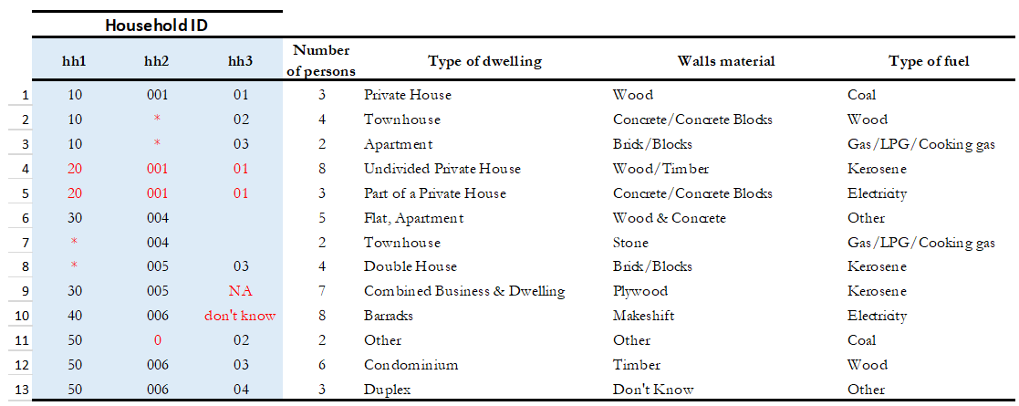
Example 3 in Section A: Data Validations in Stata provides further details and describes the steps involved in performing a validation when the identifier is made of multiple variables.

2.5. Identifying Duplicate Observations

One way to rule out problems with the unique identifier is to check if there are duplicate observations (records with identical values for all variables, not just the unique identifiers). Duplicate observations can generate erroneous analysis and cause data management problems. Some possible reasons for duplicate data are, for example, the same record being entered twice during data collection. They could also arise from an incorrect reading of the questionnaires during the scanning process if paper-based methods are being used.

Identifying duplicate observations is a crucial step. Correcting this issue may involve eliminating the duplicates from the dataset or giving them some other appropriate treatment.

Statistical packages have several commands that help identify duplicates. Table 8 shows examples of these commands in STATA, R, Python and SPSS. The STATA command -duplicates report- generates a table that summarizes the number of copies for each record (across all variables). The command -duplicates tag- allows us to distinguish between duplicates and unique observations. For more details, refer to Example 4.

Table 8. Check for duplicates observations: STATA/R/PYTHON/SPSS commands

STATA

use “household.dta”
duplicates report
duplicates tag,
generate(newvar)

R

my_data <-
load("household.rda")
household[duplicated(household),]

Python

import pandas as pd
df=pd.read_stata("household.dta")
# list all duplicated records in a dataframe
df[df.duplicated()]

SPSS

Load dataset and choose from the menu:
- Data > Identify Duplicate Cases
execute.

2.6. Ensure That Each Individual Dataset Can Be Combined into a Single Database

For organizational purposes, microdata is often stored in different datasets. Therefore, checking the relationship between the data files is an essential step to keep in mind throughout the data validation process. The role of the data producer is to store the information as efficiently as possible, which implies storing data in different files. The role of the data user is to analyse the data as holistically as possible, which could sometimes mean that they might have to join all the different data files into a single file to facilitate analysis. It is essential to ensure that each of the separate files can be combined (merged or appended depending on the case) into a single file, should the data user want to undertake this step.

Use statistical software to validate that all files can be combined into one. For a household survey, for example, verify that all records in the individual-level files have a corresponding household in the household-level master file. Also, verify that all households have at least one corresponding record in the household-roster file that lists all individuals. Below, some considerations to keep in mind before merging data files:

• The variable name of the identifier should be the same across all datasets.
• The ID variables need to be the same type (either both numeric or both string) across all databases.
• Except for ID variables, it is highly recommended that the databases don't share the same variable names or labels.

Example: Joining Household and Child Datasets

A household survey is disseminated in two datasets; one contains information about household characteristics and the other contains information on the children (administered only to mothers or caretakers). To build a dataset containing all the information about the household characteristics, including where the children live, one needs to combine these files. Users are thus assured that all observations in the child-level file have corresponding household information.

Joining data files: Hypothetical data set

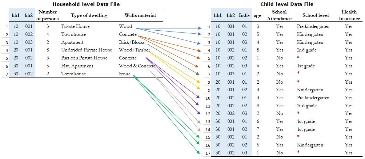
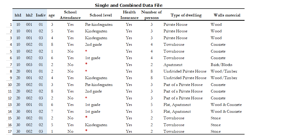
Statistical packages have some commands that allows us to combine datasets using one or multiple unique identifiers. Table 9 shows examples of these commands/functions in STATA, R and SPSS. For more details, refer to Example 5.

Table 9. Joining data files: STATA/R/PYTHON/SPSS commands

STATA

use “household.dta”
merge 1:m hh1 hh2 hh3
using
"individuals.dta"

R

household <- load("household.rda")
individuals <- load("individuals.rda")
md <- merge(household, individuals,
by = c("hh1", "hh2", “hh3”),
all =TRUE)

Python

import pandas as pd
 
household = pd.read_stata("household.dta")
individuals = pd.read_stata("individuals.dta")
 
md = pd.merge(
    household,
    individuals,
    on=["hh1", "hh2", "hh3"],
    how="outer"
)

SPSS

Load dataset and choose from the menu:
- Data > Merge Files > Add Variables
- Select the data file to merge
- Select Key Variables

Panel datasets should be stored in different files as well. Having one file per data collection period is a good practice. To combine the different periods of a panel dataset, the data user could merge them (Adding variables to the existing observations for the same period) or append them (Adding observations for a different period to the existing variables). To make sure that panels can be properly appended, the following checks are suggested:

• Check for the column(s) that identifies the period of the data (Year, Wave, Series, etc.).
• The variable names and variable types should be the same across all datasets.
• Ensure that the variables use the same label and the same coding across all datasets.

To combine datasets vertically, use the following

• SPSS: "Append new records"
• STATA: append
• Python: pd.concat(household, individuals)
• R: rbind(household, individuals) or bind_rows(household,individuals)

2.7. Check That the Data Types Are Correct

Do not include string variables if they can be converted into numeric variables. Look at your data and check the variables' types, particularly for those that you expect to be numeric (age, years, number of persons/employees/hours, income, purchases/expenditures, weights, and so forth). If there are numeric variables stored as string variables, your data needs cleaning.

For example, Table 10 contains a data set at the individual-level with some variables that should be numeric. The columns B (Age) and E (Working Weeks) are stored as numeric variables, which is fine. However, the variables 'Number of working of hours per week' (Column G), 'Number of persons working at the business' (Column H) and 'Monthly Income' (Column I) are loaded as strings because there are non-numeric values (don't know, skip, refused to answer) and some missing values present. Those variables need to be cleaned and converted from string variables to numeric variables.

Table 10. Checking Data Types: Hypothetical data set

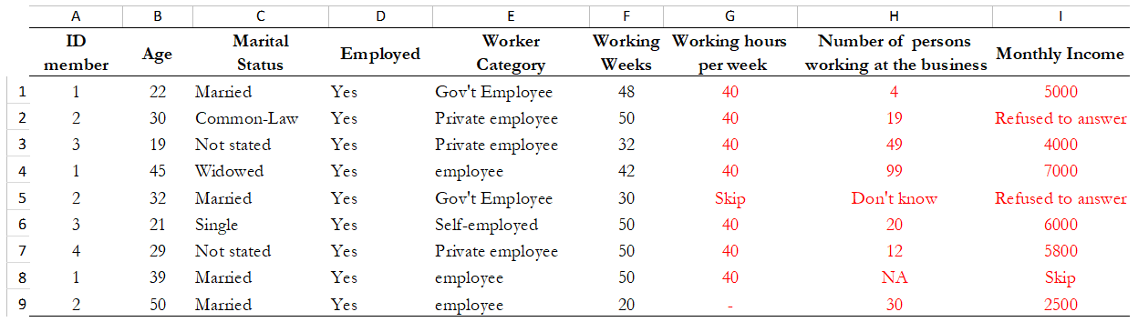
Statistical packages have some commands that allows us to make such conversions. Table 11 shows examples of these commands/functions in STATA, R, PYTHON and SPSS.

Table 11. Convert string variables to numeric: STATA/R/PYTHON/SPSS commands

STATA

use "individual.dta"
destring (varname),generate

R

individual <-
load("individual.rda")
replace}
as.numeric(individual$varname)

Python

import pandas as pd
df = pd.read_stata('individual.dta')
df["varname_num"] = pd.to_numeric(df["varname"], errors="coerce")

SPSS

Load dataset and choose from the menu:
- Data > Transform > Recode into Same individual$varname <-
- Select the variable
- Select "Old and New Values" and Recode it
- Select "Convert numeric strings to numbers ('5'->5)

2.8. Check for Variables With Missing Values

Getting data ready for documentation also involves checking for variables that do not provide complete information because they are full of missing values. This step is important because missing values can have unexpected effects on the data analysis process. Typically, missing values are defined as a character (.a, .b, single period or asterisks), special numeric (-1, -2) or blanks. Variables entirely comprised of missing values should ideally not be included in the dataset. However, before excluding them, it is useful to check whether the missing values are expected according to the questionnaire, and the skip patterns.

For example, a hypothetical household survey at the individual-level (Table 10) provides information about the respondent's employment status. The survey identifies if the respondent is employed in Column D, and then provides information about the worker category in Column E, but only for those who reported being employed in Column D. This means that those who answered 'unemployed' in column D should have a valid missing value in column E. In other words, this is a pattern in the missing values that should be observed and duly noted.

On the other hand, Columns F and G are used to determine if the people who are not employed are looking for a job and are actively seeking it. These questions are not asked to the employed people (those who answered "yes" in Column D), which mean that again, the missing values in those columns correspond with what is expected. However, Column H contains information for all employed individuals, so missing values in this column suggest that there is a problem in the data and should be addressed. Therefore, one should not blindly delete missing values at the outset without checking for these patterns.

Table 12. Checking for Missing Values: Hypothetical data set

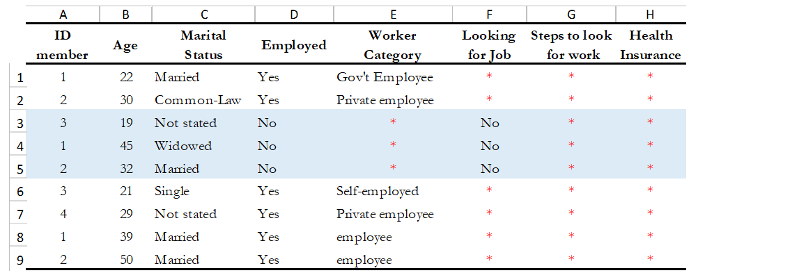
In SPSS, use the function "Missing Value Analysis" and in R, do as shown in Table 12. You can also use the STATA command -misstable summarize- that produces a report that counts all the missing values. You can also use the -rowmiss()- command with -egen- to generate the number of missing values among the specified variables. For more details, refer to Example 6.

Table 13. Counting Missing Values: STATA/R/PYTHON/SPSS commands

STATA

use “individual.dta”
misstable summarize

R

my_data <-
load("individual.rda")
colSums(is.na(individual))
colMeans(is.na(individual))

Python

import pandas as pd
df = pd.read_stata('individual.dta')
df.isna().sum()
# to see number and percentage of missing values, use:
missing = pd.DataFrame({
    "Missing": df.isna().sum(),
    "Percent": (df.isna().sum() / len(df) * 100).round(2)
    })

print(missing)

SPSS

# Load dataset and choose from the menu:
- Data > Analyze > Missing Value Analysis
- Select “Use All Variables”

Best Practices

Since there are different reasons for missing values, data producer should code them with negative integers or letters to distinguish the missing values and valid data. For instance, (− 1) might be the code for "Don't Know", (-2) the code for "Refused to Answer" and (-9) code for "Not Applicable".

2.9. Check Improper Value Ranges

It is helpful to generate descriptive statistics for all variables (frequencies for discrete variables; min/max/mean for continuous variables) and verify that these statistics look reasonable. Just as there are variables that must take on only specific values, such as "F" and "M" for gender, there are also some variables that can take on several values (such as age or height). However, those values must fit a particular range. For example, we don't expect negative values, or typically see values over 115 years for age.

Values for categorical variables should be guided by the questionnaire (or separate documentation for constructed variables). If we have an education variable that has 9 response options in the questionnaire, the corresponding 'education' variable in the dataset should have 9 categories. We should not observe more than 9 unique values for this variable. Similarly, for any questions for which the options are only "yes", "no" and "other", we should not observe more than these 3 unique values. When out of range values exist, this might signal data cleaning issues.

Table 14 shows examples of some commands/functions in STATA, R, PYTHON and SPSS.

Table 14. Generate descriptive statistics: STATA/R/PYTHON/SPSS Commands

STATA

use “individual.dta”
summarize

R

individual <-
load("individual.rda")
summary(individual)

Python

import pandas as pd
df = pd.read_stata("individual.dta")
df.describe()

SPSS

Load dataset and choose
from the menu:
- Data > Analyze > Descriptive Statistics > Frequencies
- Select “Statistics"

2.10. Verify Weights, Design Variables, and Adjustment Factors (Where Applicable)

Some microdata collections include weights, adjustment factors, or design variables that are required for producing valid estimates and analyses. Where such variables exist, verify that they are included in the dataset, clearly labeled, properly documented, and consistent with the accompanying methodology documentation.

For sample-based datasets, weighting variables are often provided to enable users to produce estimates that are representative of a larger target population. In these cases, the documentation should clearly describe how the weights were constructed, how they should be applied, and any limitations associated with their use. Basic validation checks, such as reviewing minimum and maximum values, identifying missing values, and confirming alignment with the documented methodology, can help detect potential issues.

In some datasets, adjustment factors may be included to account for non-response, calibration, post-stratification, benchmarking, or other statistical corrections. Where applicable, these factors should be clearly identifiable and adequately documented.

Not all microdata require weights. For example, administrative records, transaction data, operational systems, registries, and complete censuses may not include weighting variables because they are intended to represent the full population of interest or are not derived from a sample. However, even in these cases, any transformations, adjustment factors, or derived analytical variables used to support analysis should be documented and preserved.

Where the data are based on a sample design (surveys), verify that the variables identifying stratification levels, clusters, primary sampling units, or other design elements are included and clearly documented. These variables are often necessary for estimating sampling errors and producing statistically valid analyses.

More generally, ensure that any variables required to correctly interpret, aggregate, weight, or analyze the data are present, clearly identifiable, and accompanied by sufficient documentation to support their appropriate use by data users.

2.11. Variables and Codes for Categorical Variables Must Be Labelled

Variable Labels

Variable labels should be concise, precise, and informative. They provide a clear description of the information contained in a variable and help users understand how the data relate to the corresponding literal questions. Without meaningful variable labels, it can be difficult to interpret the contents of a dataset or link variables back to the questionnaire. Therefore, all variables should be clearly labelled.

Even when variables are labelled, the following good practices should be followed:

• Variable labels should be informative, accurate, and as concise as possible. While software packages may allow relatively long labels (for example, up to 80 characters in Stata and 255 characters in SPSS), shorter labels are generally easier to read and manage.
• Avoid using the full literal question as a variable label. Literal questions are often lengthy and may exceed recommended label lengths. Instead, provide a brief description that captures the essence of the question.
• Each variable should have a unique label. The same label should not be used for different variables, as this can create confusion and make analysis more difficult.
• Labels should clearly distinguish between related variables and use consistent terminology throughout the dataset.
• Variable labels should complement, not replace, detailed variable descriptions. While labels provide a short summary, the variable description^[2] should capture the full wording of the question, interviewer instructions, concepts being measured, derivation methods, or any other contextual information needed to interpret the data correctly.
• Well-documented labels and descriptions improve data quality by making datasets easier to understand, review, validate, and reuse. They also support metadata extraction, search, and discovery, and help automated tools accurately interpret variables and generate reliable outputs.

Value Labels

Label values are used for categorical variables. To ensure the correct encoding of data, it is important to check that the stored values in those variables correspond to what is expected according to the questionnaire. In the case of continuous variables, we also suggest the checking of ranges. For instance, if the question is about the number of working hours, the variable should not have negative values.

You can compare variable labels in the dataset to those in the questionnaire using the --codebook- Stata command or --labelbook-. Refer to Example 8 for further details.

2.12. Assess Variable Relevance

Temporary, calculated or derived variables should not be disseminated. Remove all unnecessary or temporary variables from the data files. These variables are not collected in the field and present no interest for users.

The data producer could generate variables that are only needed during the quality control process but are not relevant to the final data user. For example, the variable "merge" in Stata is generated automatically after performing the check described in the Numeral 1.6, when the data producer wants to see if the datasets match properly. Variables that group categories of a question, dummy variables that identify a question's category are all variables produced during the coding process that are not relevant once the analysis is completed.

There are cases in which calculated variables may be useful to the users, so they must be documented in the metadata. For example, most Labor Force Surveys (LFS) contain derived dummy variables to identify the sections of the population that are employed or unemployed. These variables are generated using multiple questions from the dataset and are essential elements of any LFS. Most data users prefer to make use of them instead of computing them on their own, to reduce the risk of error. This is a strong argument to make a case for keeping these variables in the dataset, despite them being a by-product of other original variables.

To be useful, those variables that remain in the dataset must be well documented, else they, they may be useless to or misunderstood by users.

2.13. Compress the Variables to Reduce the File Size

Compress the variables consist of reducing the size of the data file without loss of precision or modifying the information that it provides. Listed below are some reasons why compressing a data set may be a useful practice for at least three reasons: First, it makes faster the process of creating backups, uploading and downloading data files from your data repository or any microdata catalog. Second, it reduces the time that data users will need to spend working with the data. Additionally, it will make the data more accessible to the different type of users; sometimes the data size will impose restrictions on those users who lack high computational power. Third, it will help to free up disk space in the server where you store your data

Example: Compressing Variables to Reduce File Size

Table 15 shows two versions of one dataset that provides individual-level information about the year of the first union, age, school attendance, and health insurance. There is no difference in the appearance of both datasets. However, version 1 was saving uncompressed and version 2 compressed. In the uncompressed version, the variables "ID" and "Year" are stored as double, which means that they can store number with high decimal precision, but they are designed to only record information of integer numbers between -32,767 and 32,740. So, the compressed version changed the storage type of these variables to int and saves 6 bytes per observation. Similarly, other variables like "age" and "school attendance" are stored as a byte in the compressed version, which saves 7 bytes per observation when are compared to the uncompressed version. Let's suppose that one has a data set with 500 variables like these, the total savings would be 3,500 bytes per observation; if this data set has 50,000 observations, it means that the savings in memory space would be around 175 megabytes.

Table 15. Compressing the Variables: Hypothetical data set

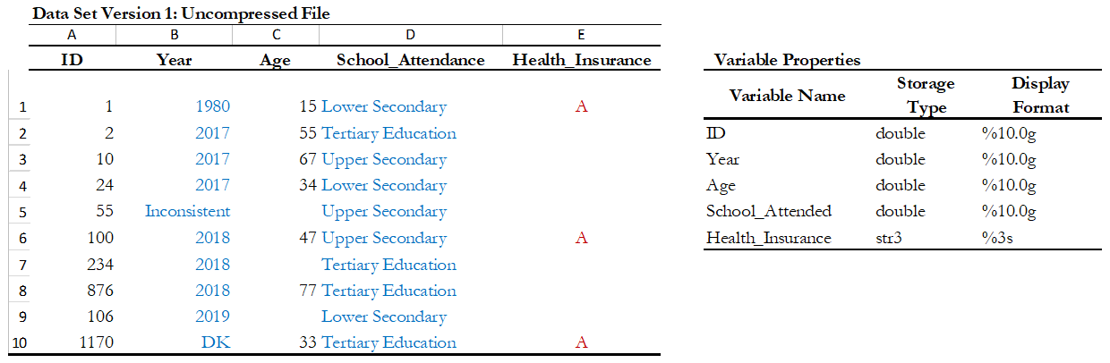
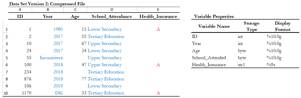
Use the compress command in Stata, or the compress option when you save a SPSS data file.

2.14. Protect respondent privacy

Keep in mind that microdata are granular data with records describing individual units such as persons, households, businesses or institutions. Because these data contain detailed information about respondents, they may pose a risk of identification or divulging sensitive information if they are not properly protected. Steps need to be taken to ensure that the privacy of respondents is protected. This is important to maintain public trust, meet ethical and legal obligations, and enable data to be shared and used responsibly for research and policy analysis.

Therefore all datasets intended to be used with automated tools, prepared for analysis, or released for dissemination must not contain direct identifiers or personally identifiable information (PII).

Before using or sharing a dataset, verify that all files have been reviewed to ensure that direct identifiers and other sensitive information that could directly or indirectly reveal the identity of respondents have been removed or treated. Examples include names, addresses, telephone numbers, email addresses, GPS coordinates, national identification numbers, and similar identifying information. Any variables containing direct identifiers should be excluded from datasets shared with others and from any datasets uploaded to online automated tools or external platforms.

If the dataset is intended for public release, it must first be transformed into an anonymous version suitable for dissemination. Removing direct identifiers is an essential first step in protecting respondent confidentiality and privacy. However, data anonymization should always begin with a careful review of the data to identify any variables that may pose a disclosure risk.

Resources to Check for PII and Apply Statistical Disclosure Control^[3] Measures

• How to search datasets for PII
• How to deidentify datasets
• An anonymization practice guide
• Introduction to the theory of anonymization for microdata
• A guide to using the graphic user interface to sdcMicro
• Introduction to Statistical Disclosure Control (SDC)

Suggestion

If you are in the process of establishing a data archive and plan to document a collection of microdata, undertake a full inventory of all existing data and metadata before you start the documentation. Use the IHSN Inventory Guidelines and Forms to facilitate this inventory (available at www.ihsn.org).

The next section focuses on organizing and preparing external resources for long-term preservation and, where appropriate, dissemination. These resources include all materials produced throughout the data lifecycle, not just the datasets themselves.

Examples include technical documentation, such as questionnaires, code lists, manuals, and methodological reports that are essential for data users; administrative and operational reports that may inform the design and implementation of future data collection projects; and supporting materials, such as stakeholder feedback, workshop proceedings, and records of decisions made during questionnaire development. Preserving these resources alongside the data helps ensure transparency, reproducibility, and the long-term value of the microdata collection.

---

1. See section 3 -- Importing data and establishing relationships for more information on key variables. ↩︎

2. See Variable Description section under Creating Structured Metadata. ↩︎

3. Statistical Disclosure Control (SDC) is the application of statistical and data modification techniques to datasets and statistical outputs to prevent the identification of individuals or organizations and the disclosure of confidential information, while maintaining the usefulness of the data for analysis. ↩︎