1. Liberia

---

Author: Andres Chamorro
Date: March 15, 2023

The objective of this analysis is to construct health facility access indicators over the general population, and across the socioeconomic distribution for a set of GFF countries with available geolocalized facility level information.

Indicators of interest

• Percentage of population within 2h of driving to the nearest primary care facility (population level, and by SES quintile).

• Percentage of population within 2h of driving to the nearest district hospital (population, and by SES quintile).

• Percentage of health facilities with direct access to an all season road.

• Percentage of health facilities within 2km of an all season road.

Data Sources

• Health facilities: National Registry Master List, we geo-coded entries with missing coordinates

• Administrative Boundaries: World Bank GAUL Level 1/2

• Global Friction Surface (2019)

• Population 2020: WorldPop 1km Grid Unconstrained

1.1. Data preparation

This first section conducts some common data preparation tasks:

• Import libraries

• Load input data (this notebook was ran from the DEC JNB server)

• Merge population and friction surface raster data

• Prepare origins (population grid) and destinations (health facilities)

Show code cell content Hide code cell content

## Define Imports

import os, sys
from os.path import join
import geopandas as gpd
import pandas as pd
import rasterio as rio
import numpy as np
from shapely.geometry import Point
import skimage.graph as graph
from rasterstats import zonal_stats

# for plotting maps
import matplotlib.pyplot as plt
import matplotlib.colors as colors
from matplotlib import colorbar
from rasterio.plot import plotting_extent
import contextily as ctx
from mpl_toolkits.axes_grid1.inset_locator import inset_axes

# for roads
import json
from utm_zone import epsg as epsg_get

# for facebook data
from pyquadkey2 import quadkey

# for graphs
from plotnine import ggplot, aes, geom_col, labs, theme_minimal, theme, element_blank, facet_wrap, scale_y_continuous
from mizani.formatters import percent_format
import seaborn as sns
import matplotlib.ticker as mtick

## TO DO: Work to consolidate functions onto a sinle package/module
sys.path.append('/home/wb514197/Repos/gostrocks/src') # gostrocks is used for some basic raster operations (clip and standardize)
sys.path.append('/home/wb514197/Repos/GOSTNets_Raster/src') # gostnets_raster has functions to work with friction surface
sys.path.append('/home/wb514197/Repos/INFRA_SAP') # only used to save some raster results

import GOSTRocks.rasterMisc as rMisc
import GOSTNetsRaster.market_access as ma
from infrasap import aggregator
from infrasap import osm_extractor as osm

## Input health and admin data

iso3 = "LBR"
input_dir = "/home/public/Data/PROJECTS/Health" #
out_folder = os.path.join(input_dir, "output", iso3)
if not os.path.exists(out_folder):
    os.mkdir(out_folder)
lbr_master = pd.read_csv(join(input_dir, "from_tashrik", "master lists", "Liberia MFL Adjusted.csv"), index_col=0)
lbr_geocoded = pd.read_csv(join(input_dir, "from_tashrik", "master lists", "Liberia MFL Adjusted Geocoded_Validated.csv"), index_col=0)

global_admin = '/home/public/Data/GLOBAL/ADMIN/g2015_0_simplified.shp'
adm0 = gpd.read_file(global_admin)
aoi = adm0.loc[adm0.ISO3166_1_==iso3]

global_admin2 = '/home/public/Data/GLOBAL/ADMIN/Admin2_Polys.shp'
adm2 = gpd.read_file(global_admin2)
adm2 = adm2.loc[adm2.ISO3==iso3].copy()
adm2 = adm2.to_crs("EPSG:4326")
adm2.reset_index(inplace=True)

## Friction Surface and Population

global_friction_surface = "/home/public/Data/GLOBAL/INFRA/FRICTION_2020/2020_motorized_friction_surface.geotiff"
global_population = "/home/public/Data/GLOBAL/Population/WorldPop_PPP_2020/ppp_2020_1km_Aggregated.tif"
inG = rio.open(global_friction_surface)

# Clip the travel raster to AOI
out_travel_surface = os.path.join(out_folder, "travel_surface.tif")
rMisc.clipRaster(inG, aoi, out_travel_surface, crop=True, buff=0.1)

inP = rio.open(global_population)

# Clip the pop raster to AOI
out_pop = os.path.join(out_folder, "WP_2020_1km.tif")
rMisc.clipRaster(inP, aoi, out_pop, crop=True, buff=0.1)

travel_surf = rio.open(out_travel_surface)
pop_surf = rio.open(out_pop)

# standardize so that they have the same number of pixels and dimensions
out_pop_surface_std = os.path.join(out_folder, "WP_2020_1km_STD.tif")
rMisc.standardizeInputRasters(pop_surf, travel_surf, out_pop_surface_std, resampling_type="nearest")

# create a data frame of all points
pop_surf = rio.open(out_pop_surface_std)
pop = pop_surf.read(1, masked=True)
indices = list(np.ndindex(pop.shape))
xys = [Point(pop_surf.xy(ind[0], ind[1])) for ind in indices]
res_df = pd.DataFrame({
    'spatial_index': indices, 
    'xy': xys, 
    'pop': pop.flatten()
})
res_df['pointid'] = res_df.index

# create MCP object
inG_data = travel_surf.read(1) * 1000 # minutes to travel 1 meter, convert to km
# Correct no data values
inG_data[inG_data < 0] = 9999999999 # untraversable
# inG_data[inG_data < 0] = np.nan
mcp = graph.MCP_Geometric(inG_data)

## Destinations
lbr = lbr_master.loc[lbr_master.functional=="functional"].copy()
lbr = lbr.loc[~(lbr.latitude.isna())].copy()
lbr_geocoded = lbr_geocoded.loc[lbr_geocoded.geocoding_method!="District name and county query"].copy()
lbr = pd.concat([lbr, lbr_geocoded])
lbr.reset_index(drop=True, inplace=True)
geoms = [Point(xy) for xy in zip(lbr.longitude, lbr.latitude)]
lbr_geo = gpd.GeoDataFrame(lbr, crs='EPSG:4326', geometry=geoms)

lbr_geo_filt = lbr_geo.loc[lbr_geo.intersects(aoi.unary_union)]
lbr_geo_filt.reset_index(inplace=True, drop=True)
hospitals = lbr_geo_filt.loc[lbr_geo_filt.facilitytype=="hospital"].copy()
# lbr_geo_filt = lbr_geo.copy()

/home/wb514197/Repos/gostrocks/src/GOSTRocks/rasterMisc.py:73: UserWarning: Geometry is in a geographic CRS. Results from 'buffer' are likely incorrect. Use 'GeoSeries.to_crs()' to re-project geometries to a projected CRS before this operation.

/home/wb514197/Repos/gostrocks/src/GOSTRocks/rasterMisc.py:73: UserWarning: Geometry is in a geographic CRS. Results from 'buffer' are likely incorrect. Use 'GeoSeries.to_crs()' to re-project geometries to a projected CRS before this operation.

Summary of health facilities by type

Show code cell source Hide code cell source

lbr_geo_filt.facilitytype.value_counts()

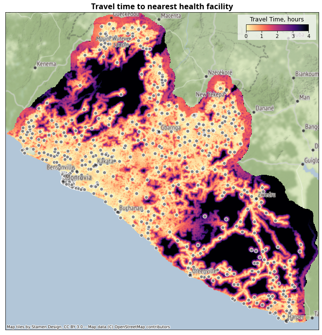
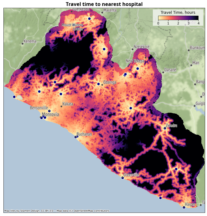
1.2. Calculate travel time to nearest health facility

We calculate driving time from every populated place (using a 1 km population grid) to the nearest health facility, using the global friction surface.​

Show code cell source Hide code cell source

## Calculate travel time to nearest health facility / hospital
res_health = ma.calculate_travel_time(travel_surf, mcp, lbr_geo_filt)[0]
res_hospital = ma.calculate_travel_time(travel_surf, mcp, hospitals)[0]

res_df.loc[:, f"tt_health"] = res_health.flatten()
res_df.loc[:, f"tt_hospital"] = res_hospital.flatten()

res_df = res_df.loc[res_df['pop']>0].copy()
res_df = res_df.loc[~(res_df['pop'].isna())].copy()
res_df.loc[:,'xy'] = res_df['xy'].apply(Point)

res_gdf = gpd.GeoDataFrame(res_df, geometry='xy', crs='EPSG:4326')
res_gdf.loc[:, 'geometry'] = res_gdf.loc[:, 'xy']

raster_path = out_pop_surface_std
aggregator.rasterize_gdf(res_gdf, 'tt_health', raster_path, os.path.join(out_folder, "tt_health_temp.tif"), nodata=-1)
aggregator.rasterize_gdf(res_gdf, 'tt_hospital', raster_path, os.path.join(out_folder, "tt_hospital_temp.tif"), nodata=-1)

tt_health_rio = rio.open(os.path.join(out_folder, "tt_health_temp.tif"))
tt_health = tt_health_rio.read(1, masked=True)

tt_hospital_rio = rio.open(os.path.join(out_folder, "tt_hospital_temp.tif"))
tt_hospital = tt_hospital_rio.read(1, masked=True)

tt_health = tt_health/60
tt_hospital = tt_hospital/60

1.2.1. Travel Time Maps

Show code cell source Hide code cell source

figsize = (12,12)
fig, ax = plt.subplots(1, 1,  figsize = figsize)
fonttitle = {'fontname':'Open Sans','weight':'bold','size':16}
ax.set_title("Travel time to nearest health facility", fontdict=fonttitle)
ax.get_xaxis().set_visible(False) # plt.axis('off')
ax.get_yaxis().set_visible(False)

vmin = 0
vmax = 4
cmap = 'magma_r'

ext = plotting_extent(tt_health_rio)
im = ax.imshow(tt_health, cmap=cmap, extent=ext, vmin=vmin, vmax=vmax) # norm=colors.PowerNorm(gamma=0.3)

orientation='horizontal'
alpha=1

cbbox = inset_axes(
    ax, '25%', '8%', loc = 'upper right'
)
cbbox.set_title('Travel Time, hours', y=1.0, pad=-14)
[cbbox.spines[k].set_visible(False) for k in cbbox.spines]
cbbox.tick_params(
    axis='both', which='both',
    left=False, top=False, right=False, bottom=False, 
    labelleft=False, labeltop=False, labelright=False, labelbottom=False
)
cbbox.set_facecolor([1,1,1,0.7])
# cbbox.set_axis_off()

cax = inset_axes(cbbox, '80%', '25%', loc = 'center')

cmap = plt.get_cmap(cmap)
norm = colors.Normalize(vmin=vmin, vmax=vmax)
cb = colorbar.ColorbarBase(
    ax=cax, norm=norm, alpha=alpha, cmap=cmap, orientation=orientation,
)

lbr_geo_filt.plot(ax=ax, facecolor='gray', edgecolor='white', markersize=50, alpha=1)
# ctx.add_basemap(ax, source=ctx.providers.Stamen.Terrain, crs='EPSG:4326', zorder=-10)
ctx.add_basemap(ax, source=ctx.providers.Stamen.TerrainLabels, crs='EPSG:4326', zorder=1)
ctx.add_basemap(ax, source=ctx.providers.Stamen.Terrain, crs='EPSG:4326', zorder=-10, alpha=0.75)

# plt.tight_layout()
plt.savefig(join(out_folder, "Friction_TT_health.png"), dpi=150, bbox_inches='tight', facecolor='white')

Show code cell source Hide code cell source

figsize = (12,12)
fig, ax = plt.subplots(1, 1,  figsize = figsize)
fonttitle = {'fontname':'Open Sans','weight':'bold','size':16}
ax.set_title("Travel time to nearest hospital", fontdict=fonttitle)
ax.get_xaxis().set_visible(False) # plt.axis('off')
ax.get_yaxis().set_visible(False)


vmin = 0
vmax = 4
cmap = 'magma_r'

ext = plotting_extent(tt_health_rio)
im = ax.imshow(tt_hospital, cmap=cmap, extent=ext, vmin=vmin, vmax=vmax) # norm=colors.PowerNorm(gamma=0.3)

orientation='horizontal'
alpha=1

cbbox = inset_axes(
    ax, '25%', '8%', loc = 'upper right'
)
cbbox.set_title('Travel Time, hours', y=1.0, pad=-14)
[cbbox.spines[k].set_visible(False) for k in cbbox.spines]
cbbox.tick_params(
    axis='both', which='both',
    left=False, top=False, right=False, bottom=False, 
    labelleft=False, labeltop=False, labelright=False, labelbottom=False
)
cbbox.set_facecolor([1,1,1,0.7])

cax = inset_axes(cbbox, '80%', '25%', loc = 'center')

cmap = plt.get_cmap(cmap)
norm = colors.Normalize(vmin=vmin, vmax=vmax)
cb = colorbar.ColorbarBase(
    ax=cax, norm=norm, alpha=alpha, cmap=cmap, orientation=orientation,
)

hospitals.plot(ax=ax, facecolor='navy', edgecolor='white', markersize=80, alpha=1)
# ctx.add_basemap(ax, source=ctx.providers.Stamen.Terrain, crs='EPSG:4326', zorder=-10)
ctx.add_basemap(ax, source=ctx.providers.Stamen.TerrainLabels, crs='EPSG:4326', zorder=1)
ctx.add_basemap(ax, source=ctx.providers.Stamen.Terrain, crs='EPSG:4326', zorder=-10, alpha=0.75)
plt.savefig(join(out_folder, "Friction_TT_hospital.png"), dpi=150, bbox_inches='tight', facecolor='white')

1.3. Summarize population within 2 hours

Show code cell source Hide code cell source

pop_120_heatlh = pop*(tt_health<=2)
pop_120_hospital = pop*(tt_hospital<=2)

zs_pop = pd.DataFrame(zonal_stats(adm2, pop.filled(), affine=pop_surf.transform, stats='sum', nodata=pop_surf.nodata)).rename(columns={'sum':'pop'})
zs_lt_120_health = pd.DataFrame(zonal_stats(adm2, pop_120_heatlh.filled(), affine=pop_surf.transform, stats='sum', nodata=pop_surf.nodata)).rename(columns={'sum':'pop_120_health'})
zs_lt_120_hospital = pd.DataFrame(zonal_stats(adm2, pop_120_hospital.filled(), affine=pop_surf.transform, stats='sum', nodata=pop_surf.nodata)).rename(columns={'sum':'pop_120_hospital'})
zs = zs_pop.join(zs_lt_120_health).join(zs_lt_120_hospital)

zs.loc[:, "health_pct"] = zs.loc[:, "pop_120_health"]/zs.loc[:, "pop"]
zs.loc[:, "hospital_pct"] = zs.loc[:, "pop_120_hospital"]/zs.loc[:, "pop"]
res = adm2.join(zs)

Summary stats

Show code cell source Hide code cell source

print(f"Summary of % of pop. within 2 hr. of health facility \n {res.health_pct.describe()}")
print(f"Summary of % of pop. within 2 hr. of hospital \n {res.hospital_pct.describe()}")

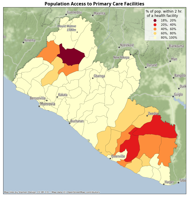
1.3.1. Accessibility Maps (Share of pop.)

Percentage of population within 2 hours of driving to the nearest primary care facility, by district (admin-2 level).​

This indicator considers clinics, health centers, and hospitals.

Show code cell source Hide code cell source

figsize = (12,12)
fig, ax = plt.subplots(1, 1,  figsize = figsize)
fonttitle = {'fontname':'Open Sans','weight':'bold','size':16}
ax.set_title("Population Access to Primary Care Facilities", fontdict=fonttitle)
ax.get_xaxis().set_visible(False) # plt.axis('off')
ax.get_yaxis().set_visible(False)

res.plot(
    ax=ax, column='health_pct', cmap='YlOrRd_r', legend=True,
    scheme='user_defined', k=5, alpha=1, linewidth=0.2, edgecolor='black', classification_kwds = {'bins': [0.2,0.4,0.6,0.8,1]},
    legend_kwds = {
        'title': "% of pop. within 2 hr. \n of a health facility", 
        'fontsize': 10,
        'fmt': "{:.0%}",
        'title_fontsize': 12
    }
)
ctx.add_basemap(ax, source=ctx.providers.Stamen.TerrainLabels, crs='EPSG:4326', zorder=1)
ctx.add_basemap(ax, source=ctx.providers.Stamen.Terrain, crs='EPSG:4326', zorder=-10, alpha=0.75)

plt.savefig(os.path.join(out_folder, "Health_Access.png"), dpi=150, bbox_inches='tight', facecolor='white')

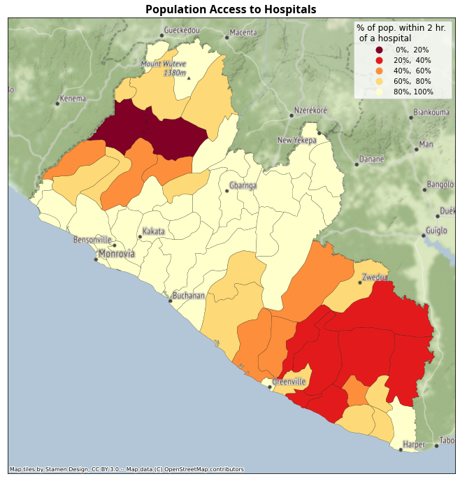
Percentage of population within 2 hours of driving to the nearest hospital, by district (admin-2 level).​

Show code cell source Hide code cell source

figsize = (12,12)
fig, ax = plt.subplots(1, 1,  figsize = figsize)
fonttitle = {'fontname':'Open Sans','weight':'bold','size':16}
ax.set_title("Population Access to Hospitals", fontdict=fonttitle)
ax.get_xaxis().set_visible(False) # plt.axis('off')
ax.get_yaxis().set_visible(False)

res.plot(
    ax=ax, column='hospital_pct', cmap='YlOrRd_r', legend=True,
    scheme='user_defined', k=5, alpha=1, linewidth=0.2, edgecolor='black', classification_kwds = {'bins': [0.2,0.4,0.6,0.8,1]},
    legend_kwds = {
        'title': "% of pop. within 2 hr. \n of a hospital", 
        'fontsize': 10,
        'fmt': "{:.0%}",
        'title_fontsize': 12
    }
)
ctx.add_basemap(ax, source=ctx.providers.Stamen.TerrainLabels, crs='EPSG:4326', zorder=1)
ctx.add_basemap(ax, source=ctx.providers.Stamen.Terrain, crs='EPSG:4326', zorder=-10, alpha=0.75)

plt.savefig(os.path.join(out_folder, "Hospitals_Access.png"), dpi=150, bbox_inches='tight', facecolor='white')

1.4. Access to roads

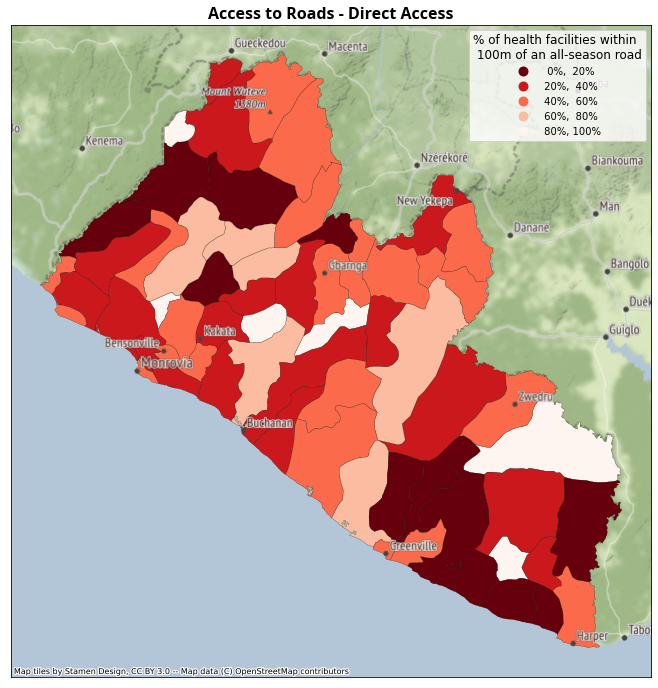
Percentage of health facilities having direct access to an all-season road, by district (admin-2 level).​

All-season road defined as primary, secondary or tertiary using the OpenStreetMap classification.​

Direct access defined as being within 100 meters of a road.​

1.4.1. Load OSM roads and define classification

{
    'motorway': 'OSMLR level 1',
    'motorway_link': 'OSMLR level 1',
    'trunk': 'OSMLR level 1',
    'trunk_link': 'OSMLR level 1',
    'primary': 'OSMLR level 1',
    'primary_link': 'OSMLR level 1',
    'secondary': 'OSMLR level 2',
    'secondary_link': 'OSMLR level 2',
    'tertiary': 'OSMLR level 2',
    'tertiary_link': 'OSMLR level 2',
    'unclassified': 'OSMLR level 3',
    'unclassified_link': 'OSMLR level 3',
    'residential': 'OSMLR level 3',
    'residential_link': 'OSMLR level 3',
    'track': 'OSMLR level 4',
    'service': 'OSMLR level 4'
}

Show code cell source Hide code cell source

roads = gpd.read_file(join(input_dir, 'osm', iso3, 'highways.shp'))

adm2_json = json.loads(adm2.to_json())
epsg = epsg_get(adm2_json)

roads = roads.to_crs(epsg)
roads['OSMLR'] = roads['type'].map(osm.OSMLR_Classes)

def get_num(x):
    try:
        return(int(x))
    except:
        return(5)
roads['OSMLR_num'] = roads['OSMLR'].apply(lambda x: get_num(str(x)[-1]))

## Calculate buffers
roads_100m = roads.copy()
roads_100m['geometry'] = roads_100m['geometry'].apply(lambda x: x.buffer(100))

roads_2km = roads.copy()
roads_2km['geometry'] = roads_2km['geometry'].apply(lambda x: x.buffer(2000))

lbr_geo_filt = lbr_geo_filt.to_crs(epsg)
# hospitals = hospitals.to_crs(epsg)

## Intersect roads and buffer
roads_1_100m = roads_100m.loc[roads_100m.OSMLR_num<=1].unary_union
roads_2_100m = roads_100m.loc[roads_100m.OSMLR_num<=2].unary_union
# roads_3 = roads.loc[roads.OSMLR_num<=3].unary_union
# roads_4 = roads.loc[roads.OSMLR_num<=4].unary_union

lbr_geo_filt.loc[:, "bool_1_100m"] = lbr_geo_filt.intersects(roads_1_100m)
lbr_geo_filt.loc[:, "bool_2_100m"] = lbr_geo_filt.intersects(roads_2_100m)
# lbr_geo_filt.loc[:, "bool_3"] = lbr_geo_filt.intersects(roads_3)
# lbr_geo_filt.loc[:, "bool_4"] = lbr_geo_filt.intersects(roads_4)

roads_1_2km = roads_2km.loc[roads_2km.OSMLR_num<=1].unary_union
roads_2_2km = roads_2km.loc[roads_2km.OSMLR_num<=2].unary_union
# roads_3 = roads.loc[roads.OSMLR_num<=3].unary_union
# roads_4 = roads.loc[roads.OSMLR_num<=4].unary_union

lbr_geo_filt.loc[:, "bool_1_2km"] = lbr_geo_filt.intersects(roads_1_2km)
lbr_geo_filt.loc[:, "bool_2_2km"] = lbr_geo_filt.intersects(roads_2_2km)
# lbr_geo_filt.loc[:, "bool_3"] = lbr_geo_filt.intersects(roads_3)
# lbr_geo_filt.loc[:, "bool_4"] = lbr_geo_filt.intersects(roads_4)

lbr_geo_filt = lbr_geo_filt.to_crs(adm2.crs)
facilities = gpd.sjoin(lbr_geo_filt, adm2[['OBJECTID', 'WB_ADM2_CO', 'geometry']], how='left')

## Get percentages
res_osmlr = facilities[['bool_1_100m','bool_2_100m','bool_1_2km','bool_2_2km','WB_ADM2_CO']].groupby('WB_ADM2_CO').sum()
res_count = facilities[['WB_ADM2_CO','bool_1_100m']].groupby('WB_ADM2_CO').count().rename(columns={'bool_1_100m':'count'})
res_osmlr_pct = res_osmlr.apply(lambda x: x/res_count['count'])

res = res.merge(res_osmlr_pct, left_on="WB_ADM2_CO", right_index=True)

1.4.2. Maps of Access to Roads

Show code cell source Hide code cell source

figsize = (12,12)
fig, ax = plt.subplots(1, 1,  figsize = figsize)
fonttitle = {'fontname':'Open Sans','weight':'bold','size':16}
ax.set_title("Access to Roads - Direct Access", fontdict=fonttitle)
ax.get_xaxis().set_visible(False) # plt.axis('off')
ax.get_yaxis().set_visible(False)

res.plot(
    ax=ax, column='bool_2_100m', cmap='Reds_r', legend=True,
    scheme='equal_interval', k=5, alpha=1, linewidth=0.2, edgecolor='black',
    legend_kwds = {
        'title': "% of health facilities within \n 100m of an all-season road", 
        'fontsize': 10,
        'fmt': "{:.0%}",
        'title_fontsize': 12
    }
)
ctx.add_basemap(ax, source=ctx.providers.Stamen.TerrainLabels, crs='EPSG:4326', zorder=1)
ctx.add_basemap(ax, source=ctx.providers.Stamen.Terrain, crs='EPSG:4326', zorder=-10, alpha=0.75)

plt.savefig(os.path.join(out_folder, "Roads_100m.png"), dpi=150, bbox_inches='tight', facecolor='white')

Show code cell source Hide code cell source

figsize = (12,12)
fig, ax = plt.subplots(1, 1,  figsize = figsize)
fonttitle = {'fontname':'Open Sans','weight':'bold','size':16}
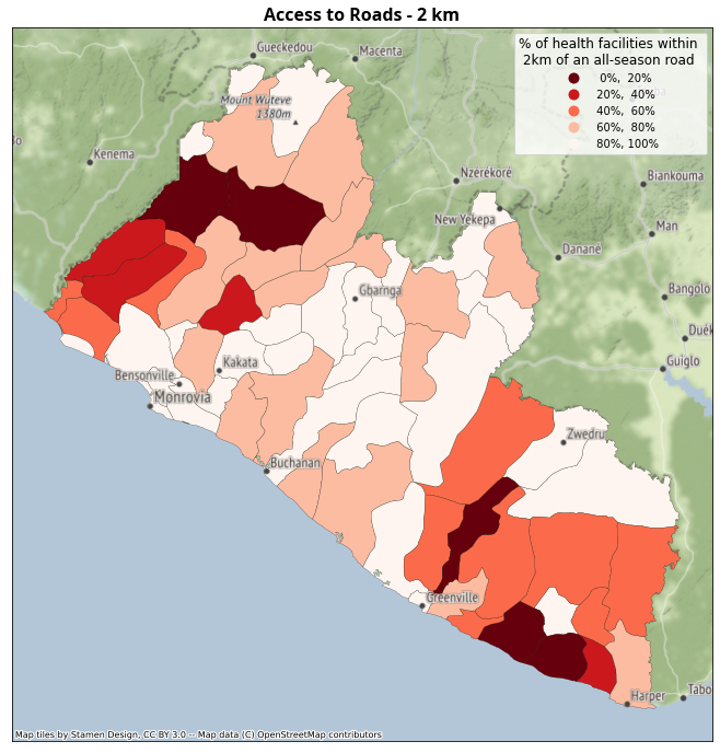
ax.set_title("Access to Roads - 2 km", fontdict=fonttitle)
ax.get_xaxis().set_visible(False) # plt.axis('off')
ax.get_yaxis().set_visible(False)

res.plot(
    ax=ax, column='bool_2_2km', cmap='Reds_r', legend=True, linewidth=0.2, edgecolor='black',
    scheme='equal_interval', k=5, alpha=1,
    legend_kwds = {
        'title': "% of health facilities within \n 2km of an all-season road", 
        'fontsize': 10,
        'fmt': "{:.0%}",
        'title_fontsize': 12
    }
)
ctx.add_basemap(ax, source=ctx.providers.Stamen.TerrainLabels, crs='EPSG:4326', zorder=1)
ctx.add_basemap(ax, source=ctx.providers.Stamen.Terrain, crs='EPSG:4326', zorder=-10, alpha=0.75)

plt.savefig(os.path.join(out_folder, "Roads_2km.png"), dpi=150, bbox_inches='tight', facecolor='white')

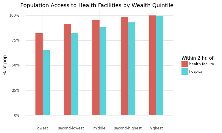
1.5. Access to health disaggregated by wealth quintile

Categorize population grid by wealth quintiles, and then summarize the population with access to health (within 2 hours of health facility or hospital)

Show code cell source Hide code cell source

fb = pd.read_csv(os.path.join(input_dir, 'facebook', 'lbr_relative_wealth_index.csv'))
fb_geoms = [Point(xy) for xy in zip(fb.longitude, fb.latitude)]
fb_geo = gpd.GeoDataFrame(fb, crs='EPSG:4326', geometry=fb_geoms)

### Summarize access with facebook grid
fb_zs = pd.DataFrame(zonal_stats(fb_geo, tt_health.filled(), affine=tt_health_rio.transform, stats='mean', nodata=tt_health_rio.nodata)).rename(columns={'mean':'tt_health'})
fb_zs_hosp = pd.DataFrame(zonal_stats(fb_geo, tt_hospital.filled(), affine=tt_hospital_rio.transform, stats='mean', nodata=tt_hospital_rio.nodata)).rename(columns={'mean':'tt_hospital'})

fb_geo = fb_geo.join(fb_zs).join(fb_zs_hosp)
fb_geo.loc[:, "rwi_cut"] = pd.qcut(fb_geo['rwi'], [0, .2, .4, .6, .8, 1.], labels=['lowest', 'second-lowest', 'middle', 'second-highest', 'highest'])
fb_geo = gpd.sjoin(fb_geo, adm2[['WB_ADM2_CO', 'WB_ADM2_NA', 'WB_ADM1_NA', 'geometry']])

### Merge population from Facebook
population = pd.read_csv(os.path.join(input_dir, 'facebook', 'population_lbr_2019-07-01.csv'))
population = population.rename(columns={'Population': 'pop_2020'})
population['quadkey'] = population.apply(lambda x: str(quadkey.from_geo((x['Lat'], x['Lon']), 14)), axis=1)

bing_tile_z14_pop = population.groupby('quadkey', as_index=False)['pop_2020'].sum()
fb_geo['quadkey'] = fb_geo.apply(lambda x: str(quadkey.from_geo((x['latitude'], x['longitude']), 14)), axis=1)
rwi = fb_geo.merge(bing_tile_z14_pop[['quadkey', 'pop_2020']], on='quadkey', how='inner')

rwi.loc[:, "tt_health_bool"] = rwi.tt_health<=2
rwi.loc[:, "tt_hospital_bool"] = rwi.tt_hospital<=2

### Aggregate at country level
rwi_pop_adm0 = rwi[['rwi_cut', 'pop_2020']].groupby(['rwi_cut']).sum()
rwi_health_adm0 = rwi.loc[rwi.tt_health_bool==True, ['rwi_cut', 'pop_2020']].groupby(['rwi_cut']).sum().rename(columns={'pop_2020':'pop_120_health'})
rwi_hospital_adm0 = rwi.loc[rwi.tt_hospital_bool==True, ['rwi_cut', 'pop_2020']].groupby(['rwi_cut']).sum().rename(columns={'pop_2020':'pop_120_hospital'})
res_rwi_adm0 = rwi_pop_adm0.join(rwi_health_adm0).join(rwi_hospital_adm0)
res_rwi_adm0.loc[:, "health_pct"] = res_rwi_adm0['pop_120_health']/res_rwi_adm0['pop_2020']
res_rwi_adm0.loc[:, "hospital_pct"] = res_rwi_adm0['pop_120_hospital']/res_rwi_adm0['pop_2020']
res_rwi_adm0.reset_index(inplace=True)

res_rwi_adm0 = res_rwi_adm0[['rwi_cut', 'health_pct', 'hospital_pct']].melt(id_vars='rwi_cut', var_name="type", value_name='pct')
res_rwi_adm0.type = res_rwi_adm0.type.str.strip("_pct")
res_rwi_adm0.loc[res_rwi_adm0.type=="health", "type"] = 'health facility'

1.5.1. Chart access to health by wealth quintile

Show code cell source Hide code cell source

(
ggplot(res_rwi_adm0, aes(x="rwi_cut", y="pct", fill="type"))
    + geom_col(width=0.5, stat='identity', position='dodge')
    + labs(
        x="", y="% of pop", title="Population Access to Health Facilities by Wealth Quintile",
        fill="Within 2 hr. of"
    )
    + theme_minimal()
    + scale_y_continuous(labels=percent_format())
    # + theme(legend_position='bottom')
)

<ggplot: (8794465317045)>

1.5.2. Aggregate to province-level (admin 1)

Show code cell source Hide code cell source

rwi_pop = rwi[['WB_ADM1_NA', 'rwi_cut', 'pop_2020']].groupby(['WB_ADM1_NA', 'rwi_cut']).sum()
rwi_health = rwi.loc[rwi.tt_health_bool==True, ['WB_ADM1_NA', 'rwi_cut', 'pop_2020']].groupby(['WB_ADM1_NA', 'rwi_cut']).sum().rename(columns={'pop_2020':'pop_120_health'})
rwi_hospital = rwi.loc[rwi.tt_hospital_bool==True, ['WB_ADM1_NA', 'rwi_cut', 'pop_2020']].groupby(['WB_ADM1_NA', 'rwi_cut']).sum().rename(columns={'pop_2020':'pop_120_hospital'})
res_rwi = rwi_pop.join(rwi_health).join(rwi_hospital)
res_rwi.reset_index(inplace=True)

res_rwi.loc[:, "health_pct"] = res_rwi['pop_120_health']/res_rwi['pop_2020']
res_rwi.loc[:, "hospital_pct"] = res_rwi['pop_120_hospital']/res_rwi['pop_2020']

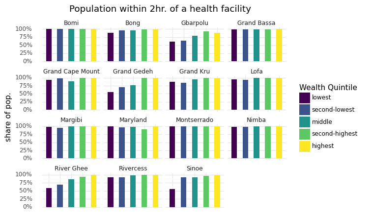
1.5.3. Chart access to health by wealth quintile, by province

Show code cell source Hide code cell source

(
ggplot(res_rwi, aes(x="rwi_cut", y="health_pct", fill="rwi_cut"))
    + geom_col(width=0.5)
    + labs(
        x="", y="share of pop.", title="Population within 2hr. of a health facility",
        fill="Wealth Quintile"
    )
    + theme_minimal()
    + theme(axis_text_x=element_blank(), axis_ticks_major_x=element_blank())
    + facet_wrap("WB_ADM1_NA")
    + scale_y_continuous(labels=percent_format())
)

<ggplot: (8794460825181)>

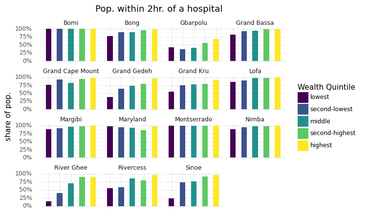
Show code cell source Hide code cell source

(
ggplot(res_rwi, aes(x="rwi_cut", y="hospital_pct", fill="rwi_cut"))
    + geom_col(width=0.5)
    + labs(
        x="", y="share of pop.", title="Pop. within 2hr. of a hospital",
        fill="Wealth Quintile"
    )
    + theme_minimal()
    + theme(axis_text_x=element_blank(), axis_ticks_major_x=element_blank())
    + facet_wrap("WB_ADM1_NA")
    + scale_y_continuous(labels=percent_format())
)

<ggplot: (8794460897181)>

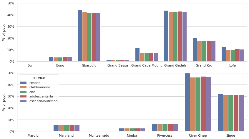
1.6. Access by Type of Service

Calculate population within 2 hours of specific health services

Show code cell source Hide code cell source

global_admin1 = '/home/public/Data/GLOBAL/ADMIN/Admin1_Polys.shp'
adm1 = gpd.read_file(global_admin1)
adm1 = adm1.loc[adm1.ISO3==iso3].copy()
adm1 = adm1.to_crs("EPSG:4326")
adm1.reset_index(inplace=True, drop=True)

tt_path = join(out_folder, 'tt_rasters')
files = [os.path.join(tt_path, f) for f in os.listdir(tt_path) if 'offer' in f]
res_tt = pd.DataFrame(zonal_stats(adm1, pop.filled(), affine=pop_surf.transform, stats='sum', nodata=pop_surf.nodata)).rename(columns={'sum':'pop'})

for f in files:
    service = f.split("_")[-1].strip('.tif')
    tt_rio = rio.open(f)
    tt = tt_rio.read(1, masked=True)
    pop_120 = pop*(tt>120)
    zs = pd.DataFrame(zonal_stats(adm1, pop_120.filled(), affine=pop_surf.transform, stats='sum', nodata=pop_surf.nodata)).rename(columns={'sum':f'{service}'})
    res_tt = res_tt.join(zs)

df = res_tt.copy()
df.reset_index(inplace=True)
df = adm1[['WB_ADM1_NA']].join(df)
df = pd.melt(df, id_vars=['index', 'WB_ADM1_NA', 'pop'], var_name='service', value_name='pop_exc')
df.loc[:, 'pop_exc_pct'] = df['pop_exc'] / df['pop']

1.6.1. Chart Access by Type of Service, province-level

Show code cell source Hide code cell source

sns.set(font_scale = 1)
sns.set_style("whitegrid")

fig, (ax1, ax2) = plt.subplots(2,1,figsize=(14,8))
sns.barplot(ax = ax1, x="WB_ADM1_NA", y="pop_exc_pct", hue="service", data=df.loc[df['index']<8])
sns.barplot(ax = ax2, x="WB_ADM1_NA", y="pop_exc_pct", hue="service", data=df.loc[df['index']>=8])
ax1.set(xlabel="", ylabel="% of pop.")
ax2.set(xlabel="", ylabel="% of pop.")
ax1.set_ylim(0, 0.5)
ax2.set_ylim(0, 0.5)
ax1.yaxis.set_major_formatter(mtick.PercentFormatter(1))
ax2.yaxis.set_major_formatter(mtick.PercentFormatter(1))
ax1.legend([],[], frameon=False)
# plt.savefig("./adm1_service.png", facecolor='white', dpi=300)

<matplotlib.legend.Legend at 0x7ff9ec585810>