Nighttime Lights Trends in Gaza and West Bank#
Analyzing conflict dynamics through the lens of NASA’s Black Marble Nighttime Lights dataset opens a unique window into the often-hidden facets of global unrest. In a world marked by diverse forms of conflict, from armed confrontations to civil unrest, the dataset offers an unconventional yet powerful tool for understanding the ripple effects of these conflicts on human settlements and infrastructure. By tracking nighttime light variations and disruptions, we can unearth vital insights into population displacement, economic destabilization, and the societal impacts of conflict. This analysis explores the potential of the Black Marble Nighttime Lights dataset to not only detect areas affected by conflict but also to quantify the extent of its influence on human lives and livelihoods, providing a valuable perspective on the multifaceted consequences of conflict worldwide.
Data#
Define Region of Interest#
Define region of interest for where NASA Black Marble will be downloaded.
Show code cell source
PSE = geopandas.read_file("../../data/boundaries/gadm41_PSE_shp/gadm41_PSE_2.shp")

PSE.explore()
Fig. 6 Region of Interest. Country borders or names do not necessarily reflect the World Bank Group’s official position. This map is for illustrative purposes and does not imply the expression of any opinion on the part of the World Bank, conceming the legal status of any country or territory or concerning the delimitation of frontiers or boundaries.#
Black Marble#
NASA’s Black Marble VIIRS (Visible Infrared Imaging Radiometer Suite) Nighttime Lights product suite represents a remarkable advancement in our ability to monitor and understand nocturnal light emissions on a global scale. By utilizing cutting-edge satellite technology and image processing techniques, the Black Marble VIIRS dataset offers a comprehensive and high-resolution view of the Earth’s nighttime illumination patterns.
VNP46A2 = bm_extract(
    PSE,
    product_id="VNP46A2",
    date_range=pd.date_range("2022-01-01", "2023-12-31", freq="D"),
    bearer=os.environ.get("BLACKMARBLE_TOKEN"),
    aggfunc=["mean", "sum"],
)
VNP46A3 = bm_extract(
    PSE,
    product_id="VNP46A3",
    date_range=pd.date_range("2022-01-01", "2023-12-31", freq="MS"),
    bearer=os.environ.get("BLACKMARBLE_TOKEN"),
    aggfunc=["mean", "sum"],
)
The latest update date is:
'08 December 2023 (Week 49)'
Important
The VNP46A2 Daily Moonlight-adjusted Nighttime Lights (NTL) Product is available daily. However, due data quality, cloud cover or other factors, the data may not be available always at a specific location.
Methodology#
Creating a time series of weekly radiance using NASA’s Black Marble data involves several steps, including data acquisition, pre-processing, zonal statistics calculation, and time series generation. Below is a general methodology for this process.
Time Series Generation#
Organize the zonal statistics results in a tabular format, where each columnn corresponds to a specific zone, and rows represent the daily radiance values. Next, we aggregate the data on a weekly basis, computing the desired statistical metric (e.g., mean radiance) for each zone for each week. Finally, we will visualize the time series data to observe trends, patterns, and anomalies over time.
Weekly#
In this step, we compute a weekly aggregation of the zonal statistics by for each second-level administrative division and for each week. In this case, we W-SUN and mean as aggregate function.
Show code cell source
PSE_2 = (
    VNP46A2.pivot_table(values=[VAR], index="date", columns=["NAME_2"])
    .resample("W-SUN", label="right")
    .mean()
)
PSE_1 = (
    VNP46A2.pivot_table(values=[VAR], index="date", columns=["NAME_1"])
    .resample("W-SUN", label="right")
    .mean()
)

PSE_2
| ntl_mean | ||||||||||||||||
|---|---|---|---|---|---|---|---|---|---|---|---|---|---|---|---|---|
| NAME_2 | Bethlehem | Deir Al-Balah | Gaza | Gaza ash Shamaliyah | Hebron | Jenin | Jericho | Jerusalem | Khan Yunis | Nablus | Qalqilya | Rafah | Ramallah and Al-Bireh | Salfit | Tubas | Tulkarm |
| date | ||||||||||||||||
| 2022-01-02 | 15.204650 | 7.979566 | 13.673667 | 8.275610 | 5.509554 | 4.963882 | 5.526086 | 26.562299 | 12.340092 | 7.097979 | 11.070501 | NaN | 9.829518 | 14.304472 | 3.700941 | 5.659215 |
| 2022-01-09 | 3.937239 | 13.335583 | 20.106966 | 12.400183 | 6.795771 | 7.521570 | 5.598589 | 21.751601 | 13.603669 | 6.986950 | 17.083686 | 22.926138 | 9.664528 | 15.148751 | 2.439910 | 11.244419 |
| 2022-01-16 | 9.067182 | 11.666783 | 15.247343 | 11.185364 | 4.952166 | 6.438554 | 4.494609 | 29.346998 | 13.005158 | 7.004429 | 14.890246 | 22.234868 | 9.463288 | 12.201209 | 1.950268 | 11.332975 |
| 2022-01-23 | 11.885563 | 13.398174 | 19.648510 | 13.627723 | 6.976829 | 7.256974 | 4.372017 | 22.756302 | 12.409488 | 7.997001 | 17.848442 | 20.634801 | 8.747132 | 13.980935 | 2.780365 | 11.759398 |
| 2022-01-30 | 3.984767 | 10.135582 | 14.438217 | 9.784870 | 4.517948 | 4.674371 | 4.451629 | 18.479181 | 10.809777 | 4.882015 | 12.376466 | 16.943309 | 6.506664 | 10.623585 | 2.216819 | 8.362207 |
| ... | ... | ... | ... | ... | ... | ... | ... | ... | ... | ... | ... | ... | ... | ... | ... | ... |
| 2023-11-12 | 7.756458 | 1.507488 | 2.757916 | 2.406718 | 10.918434 | 10.096802 | 6.133832 | 22.052848 | 1.918821 | 9.557866 | 15.885003 | 8.344134 | 10.463186 | 18.584041 | 4.042679 | 12.660648 |
| 2023-11-19 | 6.550502 | 1.168209 | 1.502485 | 3.581889 | 8.362013 | 8.276276 | 5.835015 | 26.971692 | 1.437901 | 7.638950 | 21.120911 | 4.689249 | 11.773393 | 17.621894 | 3.637760 | 15.383386 |
| 2023-11-26 | 7.156228 | 1.333906 | 1.696037 | 4.665675 | 9.008952 | 9.448789 | 6.429732 | 22.487371 | 1.634249 | 10.161027 | 18.863102 | 5.144630 | 11.334735 | 16.124129 | 3.920568 | 12.576395 |
| 2023-12-03 | 7.759852 | 0.975095 | 2.132110 | 7.532296 | 8.911090 | 9.155024 | 5.986104 | 22.749573 | 1.302449 | 8.406441 | 19.816523 | 5.199526 | 9.229725 | 19.768423 | 3.597289 | 12.000036 |
| 2023-12-10 | 5.470043 | 1.038473 | 1.294303 | 2.900198 | 8.252836 | 8.238544 | 5.389962 | 18.669865 | 1.528795 | 4.526730 | 15.682873 | 5.368840 | 8.418583 | 14.194544 | 2.411772 | 8.457151 |
102 rows × 16 columns
Monthly#
In this step, we compute a monthy aggregation of the zonal statistics by for each second-level administrative division and for each month. Additionaly, we add the VNP46A3 monthly composite, when available.
Show code cell source
p = figure(
    title="Palestine: Monthly Nighttime Lights (2022-2023)",
    width=800,
    height=600,
    x_axis_label="Date",
    x_axis_type="datetime",
    y_axis_label=r"Radiance [nW $$cm^{-2}$$ $$sr^{-1}$$]",
    tools="pan,wheel_zoom,box_zoom,reset,save,box_select",
)
p.add_layout(
    Title(
        text=f"Monthly NTL Radiance Average (VNP46A2 and VNP46A3) for each second-level administrative division",
        text_font_size="12pt",
        text_font_style="italic",
    ),
    "above",
)
p.add_layout(
    Title(
        text=f"Data Source: NASA Black Marble. Creation date: {datetime.today().strftime('%d %B %Y')}. Feedback: datalab@worldbank.org.",
        text_font_size="10pt",
        text_font_style="italic",
    ),
    "below",
)
p.add_layout(Legend(), "right")

p.add_tools(
    HoverTool(
        tooltips=[
            ("Month", "@x{%B %Y}"),
            ("Radiance", "@y{0.00}"),
        ],
        formatters={"@x": "datetime"},
    )
)
renderers = []
for column, color in zip(PSE_2_MS.columns, cc.b_glasbey_category10):
    try:
        r = p.line(
            PSE_2_MS.index,
            PSE_2_MS[column],
            legend_label=column[1],
            line_color=color,
            line_width=2,
        )
        r.visible = False
        renderers.append(r)
    except:
        pass
renderers[-1].visible = True

for column, color in zip(VNP46A3.columns, cc.b_cyclic_grey_15_85_c0):
    r = p.line(
        VNP46A3.index,
        VNP46A3[column],
        legend_label=column[1],
        line_color=color,
        line_width=2,
    )
    r.visible = False
    renderers.append(r)
renderers[-1].visible = True

p.legend.location = "bottom_left"
p.legend.click_policy = "hide"
p.title.text_font_size = "16pt"

output_notebook()
show(p)
Fig. 7 Monthly NTL radiance average derived from the VNP46A2 daily composite and, in grey, derived from the VNP46A3 monthly composite.#
Findings#
Percent Change in NTL Radiance#
Benchmark Comparison#
In this exploratory analysis, we conducted analysis of NTL radiance trends, comparing the observed average radiance levels to a benchmark established in the year 2022 for each second-level administrative division.
Show code cell source
PERCENTCHANGE_2 = 100 * (
    PSE_2 / PSE_2[(PSE_2.index >= "2022-01-01") & (PSE_2.index < "2023-01-01")].mean()
    - 1
)
PERCENTCHANGE_1 = 100 * (
    PSE_1 / PSE_1[(PSE_1.index >= "2022-01-01") & (PSE_2.index < "2023-01-01")].mean()
    - 1
)
pd.set_option("display.max_rows", None)
PERCENTCHANGE_2[PERCENTCHANGE_2.index >= "2023-10-01"].style.map(
    lambda x: "background-color: #DF4661" if x < -50 else "background-color: white"
)
| ntl_mean | ||||||||||||||||
|---|---|---|---|---|---|---|---|---|---|---|---|---|---|---|---|---|
| NAME_2 | Bethlehem | Deir Al-Balah | Gaza | Gaza ash Shamaliyah | Hebron | Jenin | Jericho | Jerusalem | Khan Yunis | Nablus | Qalqilya | Rafah | Ramallah and Al-Bireh | Salfit | Tubas | Tulkarm |
| date | ||||||||||||||||
| 2023-10-01 00:00:00 | -1.036671 | -5.176193 | -0.948034 | 17.169726 | 23.825427 | 16.148794 | 9.146616 | 13.155429 | 5.240423 | 23.910822 | -1.683530 | 6.814338 | 13.958437 | 5.481153 | 36.628251 | 1.838384 |
| 2023-10-08 00:00:00 | -15.460339 | -23.601012 | -13.217521 | 0.406629 | 22.502522 | 16.334702 | 23.188619 | -18.918551 | -19.251201 | -0.126586 | 89.428368 | -5.461336 | 4.527483 | 4.096273 | 47.435447 | 14.639749 |
| 2023-10-15 00:00:00 | -28.738148 | -84.990641 | -84.737613 | -86.295170 | 7.023393 | 16.103461 | 5.234816 | -8.937742 | -79.475160 | 5.182328 | 0.334092 | -74.805776 | 8.362368 | 6.216823 | 10.471731 | -7.134540 |
| 2023-10-22 00:00:00 | 2.589614 | -87.887605 | -85.547573 | -84.462721 | 24.019213 | 12.939151 | 17.272591 | 10.637407 | -85.656930 | 14.411997 | 9.635253 | -76.231608 | 15.861381 | 10.029488 | 27.968269 | 4.552786 |
| 2023-10-29 00:00:00 | -33.228641 | -84.899959 | -71.589192 | -79.416537 | 4.373666 | 26.021092 | 22.101463 | -38.325125 | -78.758188 | 23.409007 | 22.102664 | -68.939893 | 43.618721 | 17.616197 | 60.568520 | 12.916775 |
| 2023-11-05 00:00:00 | 31.840591 | -83.361935 | -67.098409 | -72.989751 | 31.952400 | 37.854614 | 16.826575 | 7.884103 | -76.806715 | 34.922472 | 21.287162 | -69.797142 | 28.694115 | 24.666196 | 48.756274 | 18.704953 |
| 2023-11-12 00:00:00 | 10.707432 | -88.084733 | -87.231798 | -83.939566 | 42.284195 | 31.523291 | 12.808116 | -7.058684 | -85.121654 | 19.730373 | -1.670999 | -59.688891 | 11.526984 | 29.536354 | 31.652622 | 4.416223 |
| 2023-11-19 00:00:00 | -6.505106 | -90.766412 | -93.044013 | -76.097455 | 8.970045 | 7.808694 | 7.312537 | 13.671693 | -88.850664 | -4.307680 | 30.739551 | -77.345904 | 25.492468 | 22.829905 | 18.466171 | 26.871471 |
| 2023-11-26 00:00:00 | 2.140390 | -89.456731 | -92.147935 | -68.865171 | 17.400668 | 23.082116 | 18.250061 | -5.227394 | -87.328199 | 27.286106 | 16.763595 | -75.145923 | 20.816810 | 12.390030 | 27.676013 | 3.721364 |
| 2023-12-03 00:00:00 | 10.755868 | -92.292800 | -90.129065 | -49.735730 | 16.125376 | 19.255460 | 10.091243 | -4.122347 | -89.900947 | 5.306588 | 22.665316 | -74.880719 | -1.620467 | 37.791856 | 17.148207 | -1.032048 |
| 2023-12-10 00:00:00 | -21.926431 | -91.791851 | -94.007824 | -80.646496 | 7.547307 | 7.317185 | -0.872486 | -21.316202 | -88.145879 | -43.294139 | -2.922191 | -74.062751 | -10.266420 | -1.059761 | -21.458991 | -30.251298 |
Show code cell source
show(create_plot(PERCENTCHANGE_2))
Fig. 8 Weekly percent change (compared to 2022 benchmark) in NTL radiance (VNP46A2) for each second-level administrative division.#
Additionally, we visualize below the NTL radiance average on first-level administrative division.
Fig. 9 Weekly percent change (compared to 2022 benchmark) in NTL radiance (NASA Black Marble VNP46A2) for each first-level administrative division.#
Week over Week Comparison#
In this exploratory analysis, we conducted analysis of NTL radiance trends, comparing the observed average radiance levels week over week (WOW) for each second-level administrative division.
Show code cell source
WOW_2 = 100 * (PSE_2.pct_change(1, axis="rows", fill_method=None))
Point-in-Time Comparison#
Daily#
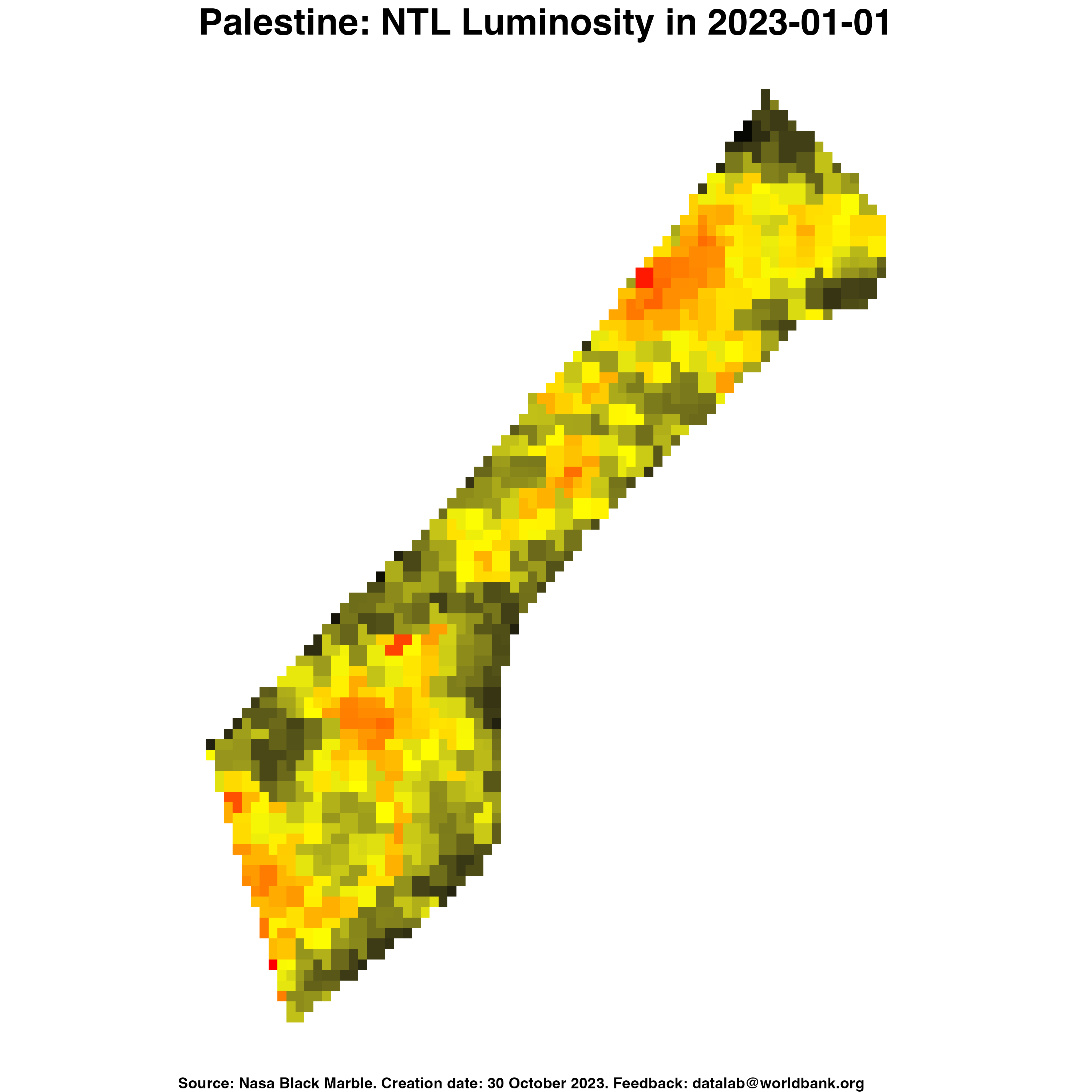
Fig. 10 Nighttime lights on January 1, 2023. Source: NASA Black Marble (VNP46A1).#
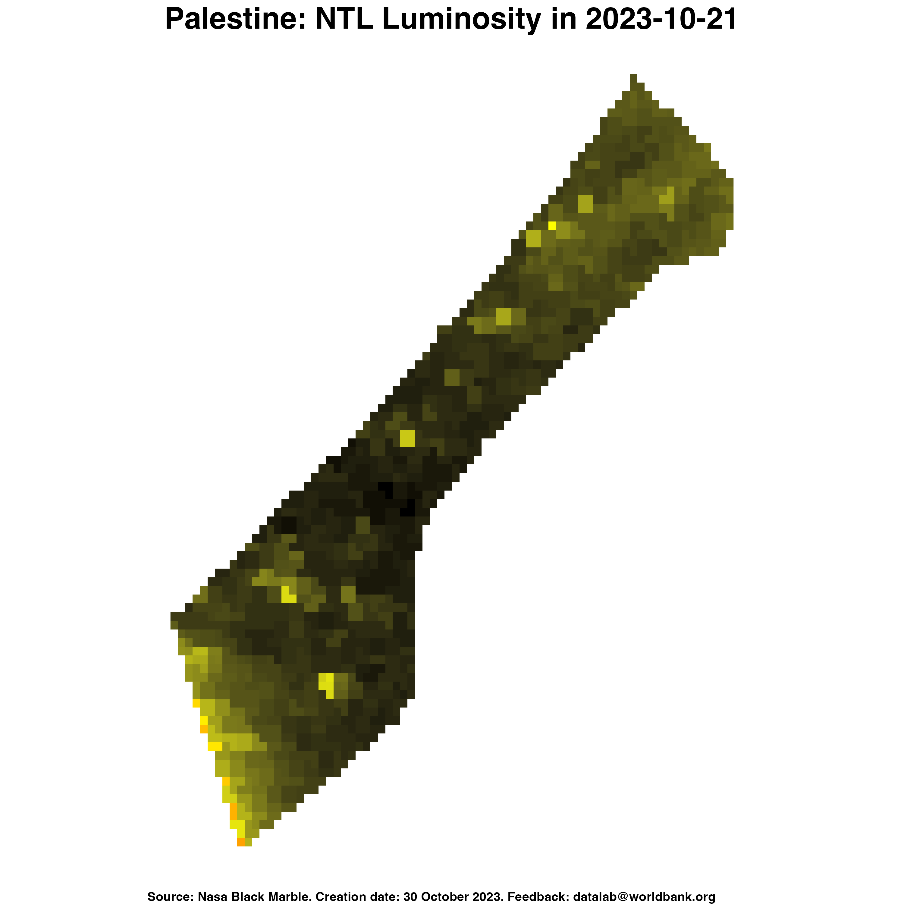
Fig. 11 Nighttime lights on October 21, 2023. Source: NASA Black Marble (VNP46A1).#
Weekly#
We visualize below weekly snapshots of the percent change (compared to 2022) in NTL radiance average for each second-level administrative division.
Limitations#
Using nighttime lights to estimate macroeconomic indicators during conflict may be a valuable approach, but it comes with several assumptions and limitations. Here’s a list of some of the key assumptions and limitations:
Caution
Assumptions:
Luminosity Reflects Economic Activity: The approach assumes that the level of nighttime lights is a reliable proxy for economic activity. It presupposes that areas with brighter lights correspond to higher economic productivity.
Baseline Data Availability: It assumes the availability of baseline nighttime lights data before the onset of the conflict. The accuracy of the estimates depends on the quality and relevance of this baseline data.
Spatial Distribution: The method assumes that nighttime lights are evenly distributed within a given geographic area and that changes in luminosity accurately reflect changes in economic activity across all locations.
Limitations:
Confounding Factors and Data Interpretation: The approach may require subjective interpretation, as it may not distinguish between reduced lighting due to conflict and reduced lighting due to other factors. Changes in nighttime lights can be influenced by factors other than economic activity, such as energy conservation measures, urban development, or seasonal variations.
Generalization: The approach might lead to overgeneralization, as a reduction in nighttime lights can be associated with various economic outcomes, from minor disruptions to severe economic downturns.
Alternative Explanations: Changes in nighttime lights can result from factors other than conflict, such as urban development, changes in economic activities, or natural disasters. Therefore, it may not always be clear whether a decline in nighttime lights is solely due to conflict.
Geopolitical Factors: The dataset may be subject to geopolitical biases, with some areas having less comprehensive coverage due to political reasons.
Data Lag: There can be a significant time lag between the occurrence of a conflict event and its reflection in the nighttime lights dataset. This lag may limit the dataset’s utility for real-time conflict monitoring.
Resolution and Urban Bias: The dataset’s spatial resolution may not be fine enough to capture small villages or isolated conflict events. It may also have an urban bias, making it less suitable for analyzing rural or remote conflicts.
To address these assumptions and limitations, it is crucial to complement nighttime lights data analysis with other sources of information and adopt a cautious and context-aware approach when interpreting the findings.
References#
- 1
Miguel O. Román, Zhuosen Wang, Qingsong Sun, Virginia Kalb, Steven D. Miller, Andrew Molthan, Lori Schultz, Jordan Bell, Eleanor C. Stokes, Bhartendu Pandey, Karen C. Seto, Dorothy Hall, Tomohiro Oda, Robert E. Wolfe, Gary Lin, Navid Golpayegani, Sadashiva Devadiga, Carol Davidson, Sudipta Sarkar, Cid Praderas, Jeffrey Schmaltz, Ryan Boller, Joshua Stevens, Olga M. Ramos González, Elizabeth Padilla, José Alonso, Yasmín Detrés, Roy Armstrong, Ismael Miranda, Yasmín Conte, Nitza Marrero, Kytt MacManus, Thomas Esch, and Edward J. Masuoka. Nasa's black marble nighttime lights product suite. Remote Sensing of Environment, 210:113–143, 2018. URL: https://www.sciencedirect.com/science/article/pii/S003442571830110X, doi:https://doi.org/10.1016/j.rse.2018.03.017.