Nighttime Lights Trends in Jordan#
The purpose of this notebook is to conduct an examination of the spatial and temporal distribution of artificial lights during the night across various regions in Jordan. The dataset utilized is derived from NASA’s Black Marble and Visible Infrared Imaging Radiometer Suite (VIIRS) on the Suomi National Polar-orbiting Partnership (Suomi NPP) satellite.
Data#
Define Region of Interest#
Define region of interest for where we want to download nighttime lights data
Show code cell source
ROI = GADMDownloader(version="4.0").get_shape_data_by_country_name(
    country_name="Jordan", ad_level=2
)
ROI.explore()
Black Marble#
NASA’s Black Marble VIIRS (Visible Infrared Imaging Radiometer Suite) Nighttime Lights dataset represents a remarkable advancement in our ability to monitor and understand nocturnal light emissions on a global scale. By utilizing cutting-edge satellite technology and image processing techniques, the Black Marble VIIRS dataset offers a comprehensive and high-resolution view of the Earth’s nighttime illumination patterns.
dates = (
    pd.date_range("2022-01-01", "2023-12-31", freq="D").strftime("%Y-%m-%d").tolist()
)
_ = bm_extract(
    roi_sf=ROI,
    product_id="VNP46A2",
    date=dates,
    bearer=os.environ.get("BLACKMARBLE_TOKEN"),
    output_location_type="file",
    file_dir="data",
    file_prefix="jor_",
    aggregation_fun=["count", "mean", "min", "max", "median", "sum"],
    quiet=True,
)
Now that the data was acquired, let’s read the data files,
Show code cell source
VNP46A2 = dd.read_csv(
    "data/jor_VNP46A2*.csv",
    parse_dates=["date"],
).compute()
VNP46A2
| ID_0 | COUNTRY | NAME_1 | NL_NAME_1 | ID_2 | NAME_2 | VARNAME_2 | NL_NAME_2 | TYPE_2 | ENGTYPE_2 | CC_2 | HASC_2 | ntl_min | ntl_max | ntl_mean | ntl_count | ntl_sum | ntl_median | date | |
|---|---|---|---|---|---|---|---|---|---|---|---|---|---|---|---|---|---|---|---|
| 0 | JOR | Jordan | Ajlun | JOR.1.1_1 | Ajloun | Ajlun | Nahia | Sub-Province | JO.AJ.AJ | 26.0 | 28.0 | 27.500000 | 4 | 110.0 | 28.0 | 2022-01-01 | |||
| 1 | JOR | Jordan | Ajlun | JOR.1.2_1 | Kofranjah | Nahia | Sub-Province | JO.AJ.KF | NaN | NaN | NaN | 0 | NaN | NaN | 2022-01-01 | ||||
| 2 | JOR | Jordan | Amman | JOR.2.1_1 | Amman | Nahia | Sub-Province | JO.AM.AM | 21.0 | 1610.0 | 305.159483 | 928 | 283188.0 | 316.0 | 2022-01-01 | ||||
| 3 | JOR | Jordan | Amman | JOR.2.2_1 | Jizeh | Al-Jiza | Nahia | Sub-Province | JO.AM.JI | 0.0 | 1072.0 | 7.873661 | 20532 | 161662.0 | 2.0 | 2022-01-01 | |||
| 4 | JOR | Jordan | Amman | JOR.2.3_1 | Mowaqqar | Al-Mwwqqar | Nahia | Sub-Province | JO.AM.MO | 3.0 | 19.0 | 12.387755 | 49 | 607.0 | 12.0 | 2022-01-01 | |||
| ... | ... | ... | ... | ... | ... | ... | ... | ... | ... | ... | ... | ... | ... | ... | ... | ... | ... | ... | ... |
| 47 | JOR | Jordan | Tafilah | JOR.11.2_1 | Hesa | Al-Hasa | Nahia | Sub-Province | JO.AT.HE | 4.0 | 113.0 | 14.097600 | 625 | 8811.0 | 11.0 | 2023-11-14 | |||
| 48 | JOR | Jordan | Tafilah | JOR.11.3_1 | Tafileh | Al-Tafila | Nahia | Sub-Province | JO.AT.AT | 8.0 | 486.0 | 31.221471 | 1332 | 41587.0 | 14.0 | 2023-11-14 | |||
| 49 | JOR | Jordan | Zarqa | JOR.12.1_1 | Azraq | Al-Azraq | Nahia | Sub-Province | JO.AZ.ZQ | 3.0 | 110.0 | 8.661039 | 3791 | 32834.0 | 8.0 | 2023-11-14 | |||
| 50 | JOR | Jordan | Zarqa | JOR.12.2_1 | Bierain | Birin | Nahia | Sub-Province | JO.AZ.BR | 23.0 | 799.0 | 123.349862 | 726 | 89552.0 | 68.0 | 2023-11-14 | |||
| 51 | JOR | Jordan | Zarqa | JOR.12.3_1 | Zarqa | Az-Zarqa | Nahia | Sub-Province | JO.AZ.AZ | 12.0 | 1625.0 | 155.380354 | 2942 | 457129.0 | 53.0 | 2023-11-14 |
34424 rows × 19 columns
The latest update date is:
'14 November 2023 (Week 46)'
Important
The VNP46A2 Daily Moonlight-adjusted Nighttime Lights (NTL) Product is available daily. However, due data quality, cloud cover or other factors, the data may not be available always at a specific location.
Methodology#
Creating a time series of weekly radiance using NASA’s Black Marble data involves several steps, including data acquisition, pre-processing, zonal statistics calculation, and time series generation. Below is a general methodology for this process.
Time Series Generation#
Organize the zonal statistics results in a tabular format, where each columnn corresponds to a specific zone, and rows represent the daily radiance values. Next, we aggregate the data on a weekly basis, computing the desired statistical metric (e.g., mean radiance) for each zone for each week. Finally, we will visualize the time series data to observe trends, patterns, and anomalies over time.
Weekly#
In this step, we compute a weekly aggregation of the zonal statistics by for each second-level administrative division and for each week. In this case, we W-SUN and mean as aggregate function.
Show code cell source
JO_2 = (
    VNP46A2.pivot_table(index="date", columns=["NAME_2"], values=[VAR]).resample("W").mean()
)

JO_1 = (
    VNP46A2.pivot_table(index="date", columns=["NAME_1"], values=[VAR], aggfunc="mean")
    .resample("W-SUN", label="right")
    .mean()
)
JO_1
| ntl_mean | ||||||||||||
|---|---|---|---|---|---|---|---|---|---|---|---|---|
| NAME_1 | Ajlun | Amman | Aqaba | Balqa | Irbid | Jarash | Karak | Ma`an | Madaba | Mafraq | Tafilah | Zarqa |
| date | ||||||||||||
| 2022-01-02 | 24.449405 | 100.560509 | 7.354693 | 69.469869 | 34.211491 | 26.072344 | 32.249152 | 14.246122 | 35.418149 | 21.112632 | 17.448854 | 27.433938 |
| 2022-01-09 | 75.069969 | 202.476405 | 8.505361 | 134.089928 | 106.841876 | 71.384097 | 27.261286 | 15.193569 | 25.749898 | 46.622935 | 21.710452 | 81.786189 |
| 2022-01-16 | 73.258399 | 146.198091 | 7.302361 | 126.774726 | 109.848380 | 70.581380 | 22.452533 | 14.715774 | 26.129812 | 41.547182 | 10.761759 | 68.849111 |
| 2022-01-23 | 66.562622 | 206.676547 | 10.440221 | 103.589737 | 101.892195 | 61.862660 | 28.897436 | 15.901350 | 22.496525 | 46.517104 | 20.465860 | 82.027899 |
| 2022-01-30 | 50.736298 | 131.449640 | 10.701375 | 110.010114 | 92.383724 | 58.473055 | 22.605634 | 13.276547 | 19.787800 | 32.544107 | 15.558135 | 51.250123 |
| ... | ... | ... | ... | ... | ... | ... | ... | ... | ... | ... | ... | ... |
| 2023-10-22 | 77.643016 | 219.769259 | 15.844977 | 131.277761 | 182.848500 | 88.222131 | 42.819114 | 23.521066 | 38.187475 | 60.871674 | 31.162284 | 105.373608 |
| 2023-10-29 | 97.636910 | 246.901782 | 14.079673 | 149.398513 | 215.814159 | 93.072254 | 43.123620 | 24.703762 | 47.732346 | 55.785789 | 31.345070 | 107.245041 |
| 2023-11-05 | 86.800853 | 217.892463 | 14.177184 | 149.693422 | 193.366805 | 93.819495 | 48.715216 | 22.026993 | 57.222549 | 67.613157 | 28.489876 | 109.128964 |
| 2023-11-12 | 79.158015 | 214.887956 | 13.880656 | 136.602316 | 167.970792 | 87.035402 | 43.076239 | 22.074731 | 51.916024 | 56.153415 | 31.205813 | 85.198662 |
| 2023-11-19 | 72.628906 | 159.532351 | 14.907425 | 96.564415 | 164.324232 | 110.157426 | 27.818617 | 21.802230 | 36.411724 | 51.083220 | 21.405399 | 72.596527 |
99 rows × 12 columns
Now, we visualize,
Show code cell source
p = figure(
    title="Jordan: Weekly Nighttime Lights (2022-2023)",
    width=800,
    height=700,
    x_axis_label="Date",
    x_axis_type="datetime",
    y_axis_label=r"Radiance [nW $$cm^{-2}$$ $$sr^{-1}$$]",
    tools="pan,wheel_zoom,box_zoom,reset,save,box_select",
)
p.add_layout(
    Title(
        text=f"Weekly Adm2 Radiance Average",
        text_font_size="12pt",
        text_font_style="italic",
    ),
    "above",
)
p.add_layout(
    Title(
        text=f"Data Source: NASA Black Marble. Creation date: {datetime.today().strftime('%d %B %Y')}. Feedback: datalab@worldbank.org.",
        text_font_size="10pt",
        text_font_style="italic",
    ),
    "below",
)
p.add_layout(Legend(), "right")

p.add_tools(
    HoverTool(
        tooltips=[
            ("Week", "@x{%W} (@x{%F})"),
            ("Radiance", "@y{0.00}"),
        ],
        formatters={"@x": "datetime"},
    )
)
renderers = []
for column, color in zip(data.columns, cc.b_glasbey_category10):
    try:
        r = p.line(
            data.index,
            data[column],
            legend_label=column[1],
            line_color=color,
            line_width=2,
        )
        r.muted = True
        renderers.append(r)
    except:
        pass

renderers[0].muted = False

p.legend.location = "bottom_left"
p.legend.click_policy = "mute"
p.title.text_font_size = "16pt"
p.sizing_mode = "scale_both"

output_notebook()
show(p)
Fig. 12 Weekly average zonal statistics (i.e., mean) for each second-level administrative division derived from NASA Black Marble.#
Monthly#
In this step, we compute a monthy aggregation of the zonal statistics by for each second-level administrative division and for each month. Additionaly, we add the VNP46A3 monthly composite, when available.
Findings#
Percent Change in NTL Radiance#
Baseline Comparison#
In this exploratory analysis, we conducted analysis of NTL radiance trends, comparing the observed average radiance levels to a baseline established in the year 2022 for each second-level administrative division.
Show code cell source
data = 100 * (
    JO_1 / JO_1[(JO_1.index >= "2022-01-01") & (JO_1.index < "2023-01-01")].mean() - 1
)

pd.set_option("display.max_rows", None)
data[data.index >= "2023-01-01"].style.map(
    lambda x: "background-color: #DF4661" if x < 0 else "background-color: white"
)
| ntl_mean | ||||||||||||
|---|---|---|---|---|---|---|---|---|---|---|---|---|
| NAME_1 | Ajlun | Amman | Aqaba | Balqa | Irbid | Jarash | Karak | Ma`an | Madaba | Mafraq | Tafilah | Zarqa |
| date | ||||||||||||
| 2023-01-01 00:00:00 | -7.812806 | -11.267915 | 5.011899 | -15.366263 | 15.477876 | -5.492497 | -23.348951 | -19.963683 | -5.625838 | -16.988747 | -29.436030 | -19.148695 |
| 2023-01-08 00:00:00 | 0.310554 | -13.267203 | 8.880067 | 11.512828 | 1.741671 | -22.658318 | -3.788541 | -13.015184 | -6.751728 | -9.967470 | -17.992759 | -15.567623 |
| 2023-01-15 00:00:00 | -1.999273 | 9.707930 | 7.380476 | 5.241753 | 12.862047 | 2.915058 | 13.266334 | -3.558661 | 7.062764 | -4.378679 | -1.982312 | 7.918166 |
| 2023-01-22 00:00:00 | 0.794651 | 5.465334 | 23.692154 | -2.033755 | 27.378690 | -0.466225 | 7.508645 | 15.741998 | -4.404656 | 8.395354 | 9.891389 | 3.479471 |
| 2023-01-29 00:00:00 | 22.966140 | -6.304200 | 3.421145 | -3.850306 | 32.130496 | 35.272439 | 5.403164 | 8.753409 | 4.319226 | -0.158464 | 9.645681 | -8.706205 |
| 2023-02-05 00:00:00 | -8.475263 | -23.819744 | 14.110618 | -18.624443 | 20.099759 | -7.395373 | -1.816518 | 11.146381 | 15.749054 | -13.603969 | -7.328799 | -12.381948 |
| 2023-02-12 00:00:00 | 16.482285 | -7.465935 | 7.813275 | -4.808203 | 2.618400 | -9.076891 | -17.564304 | 0.917458 | -4.552297 | -5.285133 | -19.107876 | -4.906531 |
| 2023-02-19 00:00:00 | 0.224380 | 5.054612 | 19.637017 | 0.749978 | 27.338746 | -0.063092 | -1.740740 | 8.707545 | 6.529947 | 6.821278 | 4.719243 | 3.467270 |
| 2023-02-26 00:00:00 | 5.688326 | 13.082583 | 25.490294 | 7.698806 | 32.034632 | 8.092545 | 18.778270 | 23.435275 | 16.031405 | 14.975504 | 15.454432 | 8.446943 |
| 2023-03-05 00:00:00 | 12.107803 | 13.855799 | 14.869858 | 10.190753 | 41.439059 | 11.703403 | 15.785757 | 17.540018 | 5.705839 | 14.346301 | 15.188396 | 10.355823 |
| 2023-03-12 00:00:00 | 5.394269 | 1.948534 | 1.515720 | -0.844330 | 26.102329 | -4.048381 | 3.092359 | 0.574206 | -4.533436 | 11.560730 | -1.378952 | 1.780216 |
| 2023-03-19 00:00:00 | -5.950738 | -37.443196 | -4.374279 | -25.656802 | 16.850970 | -29.256450 | -7.043793 | -6.737590 | -20.492548 | -16.573866 | -18.564680 | -11.080243 |
| 2023-03-26 00:00:00 | 2.840896 | -55.335895 | -27.086912 | -30.515443 | -10.117618 | 54.569092 | -22.450259 | -44.801891 | -32.930745 | -45.436535 | -48.948417 | -40.717521 |
| 2023-04-02 00:00:00 | -8.075619 | 7.384276 | 3.990688 | -2.304129 | 17.187963 | -0.575286 | 0.098759 | 8.529672 | 1.515720 | -1.971939 | -2.010714 | 11.396500 |
| 2023-04-09 00:00:00 | 2.351525 | -10.766051 | 5.863195 | 11.087220 | 42.417099 | 1.246009 | -13.201905 | -18.461676 | 1.678231 | -12.909904 | -17.918398 | -7.619874 |
| 2023-04-16 00:00:00 | 10.366028 | 28.214882 | 22.987737 | 14.594187 | 26.919998 | -5.691435 | -6.164979 | 15.910385 | -8.104481 | -0.127800 | 9.183503 | 18.650822 |
| 2023-04-23 00:00:00 | 19.642708 | 18.146151 | 36.312604 | -3.720045 | 46.695450 | 6.263230 | -6.254941 | 7.651540 | -10.296086 | 14.678273 | -7.306255 | 21.608081 |
| 2023-04-30 00:00:00 | 10.077350 | 17.930656 | 40.305952 | 11.107766 | 30.947302 | -0.160790 | 13.895862 | 21.702542 | 12.969900 | 18.467915 | 11.477825 | 3.682010 |
| 2023-05-07 00:00:00 | 11.571941 | 16.428437 | -5.910608 | 9.845804 | 48.207320 | 9.020242 | 18.398227 | 7.148590 | 17.560376 | 20.120525 | 7.684301 | 17.713424 |
| 2023-05-14 00:00:00 | 8.684018 | 12.564918 | 27.959567 | 7.122437 | 38.900676 | 9.215696 | 18.155957 | 22.679487 | 15.283112 | 18.247007 | 24.050749 | 15.901880 |
| 2023-05-21 00:00:00 | 21.066472 | -13.502072 | 16.166015 | 0.067031 | 22.959011 | 0.393036 | 28.859993 | 18.384918 | 23.536352 | 1.264218 | 1.886673 | 6.044839 |
| 2023-05-28 00:00:00 | 23.018605 | -11.291191 | 9.477632 | -9.465982 | 48.959064 | 4.055497 | 16.397785 | -14.013952 | 203.154412 | 30.317643 | -10.678348 | 72.558543 |
| 2023-06-04 00:00:00 | 14.150904 | -20.728678 | 31.509074 | 3.279296 | 48.977604 | -6.031027 | -5.881070 | 1.002130 | 10.550384 | 0.039403 | -12.596003 | -14.963563 |
| 2023-06-11 00:00:00 | -0.663030 | -24.739753 | -11.562115 | -7.322258 | 37.767790 | 7.792958 | -5.210806 | 8.918531 | -2.505512 | -7.049062 | 4.612522 | -19.854974 |
| 2023-06-18 00:00:00 | 7.152571 | 9.210617 | 22.961072 | 5.172324 | 43.171203 | 7.388784 | 18.657965 | 27.151520 | 12.446165 | 13.300487 | 15.613746 | 14.613685 |
| 2023-06-25 00:00:00 | 16.085599 | 24.776097 | 29.811833 | 18.735093 | 60.080565 | 17.613060 | 35.283201 | 45.131891 | 31.217755 | 27.119625 | 39.689302 | 23.620913 |
| 2023-07-02 00:00:00 | 11.861065 | 26.769801 | 23.327234 | 16.212974 | 61.980412 | 16.052084 | 32.077241 | 32.451992 | 30.947730 | 23.972545 | 29.841410 | 22.387185 |
| 2023-07-09 00:00:00 | 9.791064 | 21.502917 | -10.434832 | 14.795023 | 55.920524 | 13.380661 | 24.392512 | 17.624922 | 27.290106 | 19.913178 | 17.225915 | 18.597331 |
| 2023-07-16 00:00:00 | 14.899991 | 24.901712 | 28.963520 | 18.009265 | 63.479834 | 21.293432 | 38.085529 | 36.128461 | 36.712364 | 29.972402 | 34.565019 | 25.065108 |
| 2023-07-23 00:00:00 | 10.525418 | 20.998619 | 14.029224 | 16.068273 | 61.017530 | 16.310987 | 35.270106 | 36.295866 | 29.267635 | 21.041429 | 34.688737 | 16.782252 |
| 2023-07-30 00:00:00 | 8.410279 | 11.510949 | 11.666990 | 10.364857 | 52.120403 | 12.221718 | 27.946143 | 25.196635 | 28.491320 | 12.351011 | 23.049932 | 2.021945 |
| 2023-08-06 00:00:00 | 11.626558 | 26.748466 | -0.813060 | 19.229593 | 63.169194 | 18.954469 | 29.807447 | 22.621822 | 36.018049 | 22.668215 | 20.130139 | 21.334769 |
| 2023-08-13 00:00:00 | 8.938028 | 18.536046 | 11.621447 | 16.119576 | 49.582000 | 15.776598 | 33.554970 | 24.127700 | 41.303692 | 21.655611 | 31.651211 | 13.782232 |
| 2023-08-20 00:00:00 | 9.727200 | 5.138653 | 31.365770 | 3.660849 | -11.293947 | 5.381467 | 35.637040 | 20.826355 | 28.648537 | 0.815420 | 36.698685 | 22.819132 |
| 2023-08-27 00:00:00 | 14.288512 | 23.481603 | 26.747796 | 17.511957 | 53.661142 | 15.887500 | 46.871775 | 38.395901 | 48.068306 | 26.023789 | 46.593513 | 21.804700 |
| 2023-09-03 00:00:00 | 6.786921 | 16.420124 | -1.792705 | 8.774296 | 46.005542 | 5.012247 | 28.874166 | 11.159174 | 34.305456 | 16.870776 | 22.083313 | 12.864210 |
| 2023-09-10 00:00:00 | 9.932847 | 16.399821 | 14.885153 | 15.207731 | 50.192367 | 9.713189 | 34.205157 | 27.647360 | 42.889164 | 20.178395 | 35.635736 | 13.883222 |
| 2023-09-17 00:00:00 | 8.217128 | 14.653434 | 36.145995 | 12.121611 | 48.946089 | 9.773262 | 44.768990 | 38.358748 | 38.885765 | 22.621559 | 47.596291 | 13.957718 |
| 2023-09-24 00:00:00 | 16.132598 | 23.016463 | 34.046969 | 17.972179 | 50.974766 | 15.429908 | 46.393519 | 43.962337 | 48.049915 | 31.678748 | 52.680622 | 21.018734 |
| 2023-10-01 00:00:00 | 9.852405 | 36.062499 | 17.722342 | 12.067878 | 31.837164 | 6.651293 | 52.236428 | -1.351363 | 32.949964 | 13.746775 | 61.030612 | 42.777288 |
| 2023-10-08 00:00:00 | 15.805814 | -14.220051 | -1.777032 | 12.616470 | 7.789635 | -8.734124 | -2.006238 | -11.923738 | 45.516018 | -7.050917 | 13.365658 | -7.437438 |
| 2023-10-15 00:00:00 | 4.469029 | 38.082293 | 41.839918 | -4.531574 | 36.478126 | 1.173103 | 40.234096 | 33.533505 | 28.659335 | 18.330102 | 38.775023 | -6.411329 |
| 2023-10-22 00:00:00 | 8.547505 | 13.194416 | 44.545363 | 5.866359 | 45.229534 | 11.573335 | 30.330205 | 41.536058 | 30.550197 | 21.512497 | 50.077795 | 24.344041 |
| 2023-10-29 00:00:00 | 36.499631 | 27.169301 | 28.441421 | 20.479481 | 71.412890 | 17.707220 | 31.257042 | 48.652834 | 63.180913 | 11.360016 | 50.958092 | 26.552388 |
| 2023-11-05 00:00:00 | 21.350465 | 12.227754 | 29.330968 | 20.717306 | 53.583820 | 18.652245 | 48.276399 | 32.545595 | 95.624743 | 34.969898 | 37.207460 | 28.775476 |
| 2023-11-12 00:00:00 | 10.665524 | 10.680251 | 26.625893 | 10.160242 | 33.412743 | 10.072495 | 31.112825 | 32.832857 | 77.483510 | 12.093873 | 50.287429 | 0.536996 |
| 2023-11-19 00:00:00 | 1.537614 | -17.831222 | 35.992569 | -22.127534 | 30.516420 | 39.314606 | -15.327392 | 31.193103 | 24.479499 | 1.972712 | 3.088563 | -14.333905 |
Fig. 13 Percent change compared to a 2022 baseline. Values in red indicate a negative percent change.#
Show code cell source
p = figure(
    title="Jordan: Percent Change in Nighttime Lights Radiance",
    width=800,
    height=800,
    x_axis_label="Date",
    x_axis_type="datetime",
    y_axis_label="Radiance Percent Change (%)",
    tools="pan,wheel_zoom,box_zoom,reset,save,box_select",
)
p.xaxis.major_label_orientation = math.pi / 4
p.add_layout(
    Title(
        text=f"Percent change (compared to 2022) in NTL radiance for each second-level administrative division",
        text_font_size="12pt",
        text_font_style="italic",
    ),
    "above",
)
p.add_layout(
    Title(
        text=f"Source: NASA Black Marble. Creation date: {datetime.today().strftime('%d %B %Y')}. Feedback: datalab@worldbank.org.",
        text_font_size="10pt",
        text_font_style="italic",
    ),
    "below",
)
p.add_layout(Legend(), "right")
p.renderers.extend(
    [
        Span(
            location=datetime(2023, 10, 7),
            dimension="height",
            line_color="gray",
            line_width=1.5,
            line_dash=(4, 4),
        ),
    ]
)
p.add_tools(
    HoverTool(
        tooltips=[
            ("Week", "@x{%W} (@x{%F})"),
            ("Percent Change", "@y{0.00}% (2022 baseline)"),
        ],
        formatters={"@x": "datetime"},
    )
)
renderers = []
for column, color in zip(data.columns, cc.b_glasbey_category10):
    r = p.line(
        data.index,
        data[column],
        legend_label=str(column[1]),
        line_color=color,
        line_width=2,
    )
    r.visible = False
    renderers.append(r)

renderers[0].visible = True

p.legend.location = "bottom_left"
p.legend.click_policy = "hide"
p.title.text_font_size = "12pt"
p.sizing_mode = "scale_both"

show(p)
Fig. 14 Percent change in average Nighttime Lights (NTL) radiance over time compared to a 2022 baseline average, with a dashed line indicating October 7th.#
Week over Week Comparison#
In this exploratory analysis, we conducted analysis of NTL radiance trends, comparing the observed average radiance levels week over week (WOW) for each second-level administrative division.
Show code cell source
p = figure(
    title="Jordan: Percent Change in Nighttime Lights Radiance",
    width=800,
    height=800,
    x_axis_label="Date",
    x_axis_type="datetime",
    y_axis_label="Radiance Percent Change (%)",
    tools="pan,wheel_zoom,box_zoom,reset,save,box_select",
)
p.xaxis.major_label_orientation = math.pi / 4
p.add_layout(
    Title(
        text=f"Percent change week over week in NTL radiance for each second-level administrative division",
        text_font_size="12pt",
        text_font_style="italic",
    ),
    "above",
)
p.add_layout(
    Title(
        text=f"Source: NASA Black Marble. Creation date: {datetime.today().strftime('%d %B %Y')}. Feedback: datalab@worldbank.org.",
        text_font_size="10pt",
        text_font_style="italic",
    ),
    "below",
)
p.add_layout(Legend(), "right")
p.renderers.extend(
    [
        Span(
            location=datetime(2023, 10, 7),
            dimension="height",
            line_color="gray",
            line_width=1.5,
            line_dash=(4, 4),
        ),
    ]
)
p.add_tools(
    HoverTool(
        tooltips=[
            ("Week", "@x{%W} (@x{%F})"),
            ("Percent Change", "@y{0.00}% (WOW)"),
        ],
        formatters={"@x": "datetime"},
    )
)
renderers = []
for column, color in zip(data.columns, cc.b_glasbey_category10):
    r = p.line(
        data.index,
        data[column],
        legend_label=str(column[1]),
        line_color=color,
        line_width=2,
    )
    r.visible = False
    renderers.append(r)

renderers[0].visible = True

p.legend.location = "bottom_left"
p.legend.click_policy = "hide"
p.title.text_font_size = "12pt"
p.sizing_mode = "scale_both"

show(p)
Fig. 15 Percent change in average Nighttime Lights (NTL) radiance week over week, with a dashed line indicating October 7th.#
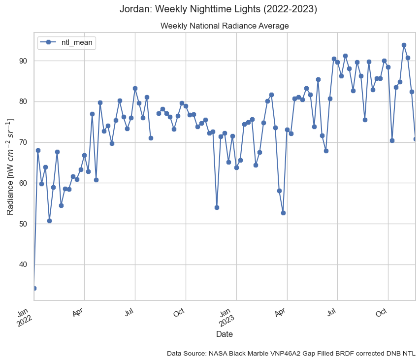
National Average Weekly Radiance#
Limitations#
See also