Assessing Quality of Nighttime Lights Data#
Overview #
The quality of nighttime lights data can be impacted by a number of factors, particularly cloud cover. To facilitate analysis using high quality data, Black Marble (1) marks the quality of each pixel and (2) in some cases of poor quality pixels, Black Marble will use data from a previous date to fill the value—using a temporally-gap filled NTL value. Below we illustrate how to examine the quality of nighttime lights data.
Setup #
We first load packages and obtain a polygon for a region of interest; for this example, we use Switzerland.
bearer = os.getenv("BLACKMARBLE_TOKEN")
gdf = geopandas.read_file(
    "https://geodata.ucdavis.edu/gadm/gadm4.1/json/gadm41_CHE_0.json"
)
gdf.explore()
Daily Data #
Below shows an example examining quality for daily data (VNP46A2).
Nighttime Lights #
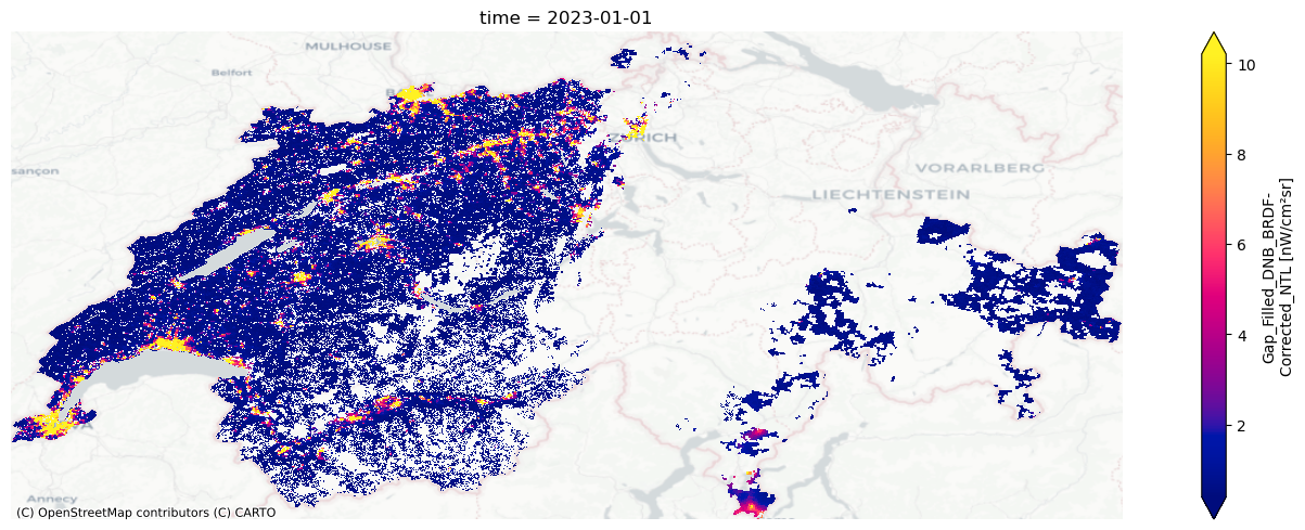
We download data for January 1st, 2023. When the variable parameter is not specified, bm_raster creates a raster using the Gap_Filled_DNB_BRDF-Corrected_NTL variable for daily data.
ntl_r = bm_raster(
    gdf,
    product_id="VNP46A2",
    date_range="2023-01-01",
    token=bearer,
    variable="Gap_Filled_DNB_BRDF-Corrected_NTL",
)
fig, ax = plt.subplots()

ntl_r["Gap_Filled_DNB_BRDF-Corrected_NTL"].sel(time="2023-01-01").plot(
    robust=True, cmap="cividis"
)
cx.add_basemap(ax, crs=gdf.crs.to_string(), source=cx.providers.CartoDB.Positron)

plt.axis("off")
plt.tight_layout()
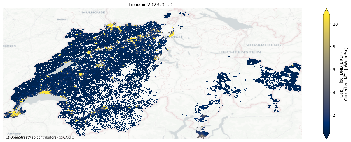
We notice that a number of observations are missing, that are poor quality and are not gap-filled. To understand the extent of missing date, we can use the following code to determine (1) the total number of pixels that cover Switzerland, (2) the total number of non-NA nighttime light pixels, and (3) the proportion of non-NA pixels.
ntl_np = ntl_r["Gap_Filled_DNB_BRDF-Corrected_NTL"].sel(time="2023-01-01")

n_pixel = zonal_stats(
    gdf,
    ntl_np.values,
    affine=transform(ntl_np),
    nodata=np.nan,
    masked=False,
    stats=["count", "nan"],
)
## Number of pixels
n_pixel[0]["count"] + n_pixel[0]["nan"]
280710.0
## Number of non nan pixels
n_pixel[0]["count"]
120565
## Proportion of non nan pixels
n_pixel[0]["count"] / (n_pixel[0]["count"] + n_pixel[0]["nan"])
0.4295001959317445
By default, bm_extract computes the mean; we can easily also compute the number of pixels and number of nan pixels.
date_range = pd.date_range(
    "2023-01-01",
    "2023-01-10",
    freq="D",
)
ntl_df = bm_extract(
    roi=gdf,
    product_id="VNP46A2",
    date_range=date_range,
    token=bearer,
    variable="Gap_Filled_DNB_BRDF-Corrected_NTL",
    aggfunc=["mean", "count", "nan"],
)
[2024-02-15 14:08:40 - backoff:105 - INFO] Backing off get_url(...) for 0.7s (httpx.ReadTimeout)
[2024-02-15 14:08:40 - backoff:105 - INFO] Backing off get_url(...) for 0.2s (httpx.ReadTimeout)
ntl_df["prop_non_na_pixels"] = ntl_df["ntl_count"] / (
    ntl_df["ntl_count"] + ntl_df["ntl_nan"]
)
ntl_df
| GID_0 | COUNTRY | geometry | ntl_mean | ntl_count | ntl_nan | date | prop_non_na_pixels | |
|---|---|---|---|---|---|---|---|---|
| 0 | CHE | Switzerland | MULTIPOLYGON (((7.04510 45.95730, 7.02940 45.9... | 1.511901 | 120565 | 160145.0 | 2023-01-01 | 0.429500 |
| 0 | CHE | Switzerland | MULTIPOLYGON (((7.04510 45.95730, 7.02940 45.9... | 1.352877 | 133176 | 147534.0 | 2023-01-02 | 0.474426 |
| 0 | CHE | Switzerland | MULTIPOLYGON (((7.04510 45.95730, 7.02940 45.9... | 0.699065 | 9732 | 270978.0 | 2023-01-03 | 0.034669 |
| 0 | CHE | Switzerland | MULTIPOLYGON (((7.04510 45.95730, 7.02940 45.9... | 1.132924 | 125537 | 155173.0 | 2023-01-04 | 0.447212 |
| 0 | CHE | Switzerland | MULTIPOLYGON (((7.04510 45.95730, 7.02940 45.9... | 0.369400 | 7245 | 273465.0 | 2023-01-05 | 0.025810 |
| 0 | CHE | Switzerland | MULTIPOLYGON (((7.04510 45.95730, 7.02940 45.9... | 1.200263 | 124697 | 156013.0 | 2023-01-06 | 0.444220 |
| 0 | CHE | Switzerland | MULTIPOLYGON (((7.04510 45.95730, 7.02940 45.9... | 1.021223 | 88498 | 192212.0 | 2023-01-07 | 0.315265 |
| 0 | CHE | Switzerland | MULTIPOLYGON (((7.04510 45.95730, 7.02940 45.9... | 1.158678 | 120015 | 160695.0 | 2023-01-08 | 0.427541 |
| 0 | CHE | Switzerland | MULTIPOLYGON (((7.04510 45.95730, 7.02940 45.9... | 1.643992 | 25566 | 255144.0 | 2023-01-09 | 0.091076 |
| 0 | CHE | Switzerland | MULTIPOLYGON (((7.04510 45.95730, 7.02940 45.9... | 1.679899 | 40913 | 239797.0 | 2023-01-10 | 0.145748 |
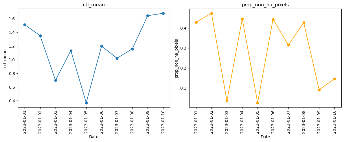
The below figure shows trends in average nighttime lights (left) and the proportion of the country with a value for nighttime lights (right). For some days, low number of pixels corresponds to low nighttime lights (eg, January 3 and 5th); however, for other days, low number of pixels corresponds to higher nighttime lights (eg, January 9 and 10). On January 3 and 5, missing pixels could have been over typically high-lit areas (eg, cities)—while on January 9 and 10, missing pixels could have been over typically lower-lit areas.
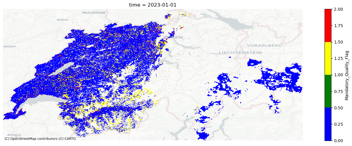
Quality #
For daily data, the quality values are:
0: High-quality, Persistent nighttime lights
1: High-quality, Ephemeral nighttime Lights
2: Poor-quality, Outlier, potential cloud contamination, or other issues
255: No retrieval, Fill value (masked out on ingestion)
We can map quality by using the Mandatory_Quality_Flag variable.
quality_r = bm_raster(
    gdf,
    product_id="VNP46A2",
    date_range="2023-01-01",
    token=bearer,
    variable="Mandatory_Quality_Flag",
)
Nighttime lights for good quality observations #
The quality_flag_rm parameter determines which pixels are set to NA based on the quality indicator. By default, only pixels with a value of 255 are filtered out. However, if we only want data for good quality pixels, we can adjust the quality_flag_rm parameter.
ntl_good_qual_r = bm_raster(
    gdf,
    product_id="VNP46A2",
    date_range="2023-01-01",
    token=bearer,
    variable="Gap_Filled_DNB_BRDF-Corrected_NTL",
    quality_flag_rm=[2, 255],
)
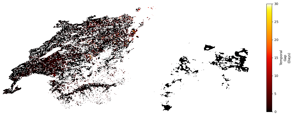
Nighttime lights for good quality observations, without gap filling #
By default, the bm_raster function uses the Gap_Filled_DNB_BRDF-Corrected_NTL variable for daily data. Gap filling indicates that some poor quality pixels use data from a previous date; the Latest_High_Quality_Retrieval indicates the date the nighttime lights value came from.
ntl_tmp_gap_r = bm_raster(
    gdf,
    product_id="VNP46A2",
    date_range="2023-01-01",
    token=bearer,
    variable="Latest_High_Quality_Retrieval",
)
r_np = ntl_tmp_gap_r["Latest_High_Quality_Retrieval"].sel(time="2023-01-01")
r_np = np.where(r_np == 255, np.nan, r_np)

plt.imshow(r_np, cmap=cc.cm.fire)
plt.axis("off")
plt.colorbar(
    label="Temporal\nGap\n(Days)"
)  # Add a colorbar with ticks for discrete values
plt.tight_layout()
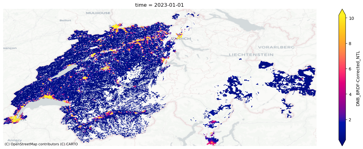
Instead of using Gap_Filled_DNB_BRDF-Corrected_NTL, we could ignore gap filled observations—using the DNB_BRDF-Corrected_NTL variable. Here, we also remove poor quality pixels.
ntl_r = bm_raster(
    gdf,
    product_id="VNP46A2",
    date_range="2023-01-01",
    token=bearer,
    variable="DNB_BRDF-Corrected_NTL",
    quality_flag_rm=[2, 255],
)
Monthly/Annual Data #
Below shows an example examining quality for monthly data (VNP46A3). The same approach can be used for annual data (VNP46A4); the variables are the same for both monthly and annual data.
Nighttime Lights #
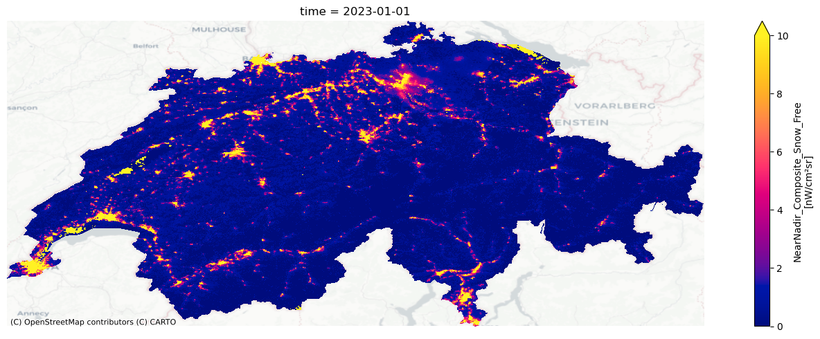
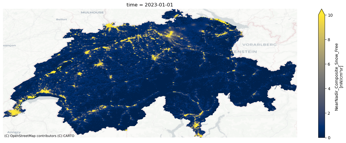
We download data for January 2023. When the variable parameter is not specified, bm_raster creates a raster using the NearNadir_Composite_Snow_Free variable for monthly and annual data—which is nighttime lights, removing effects from snow cover.
ntl_r = bm_raster(
    gdf,
    product_id="VNP46A3",
    date_range="2023-01-01",
    token=bearer,
    variable="NearNadir_Composite_Snow_Free",
)
fig, ax = plt.subplots()

ntl_r["NearNadir_Composite_Snow_Free"].sel(time="2023-01-01").plot(
    robust=True, cmap="cividis"
)
cx.add_basemap(ax, crs=gdf.crs.to_string(), source=cx.providers.CartoDB.Positron)

plt.axis("off")
plt.tight_layout()
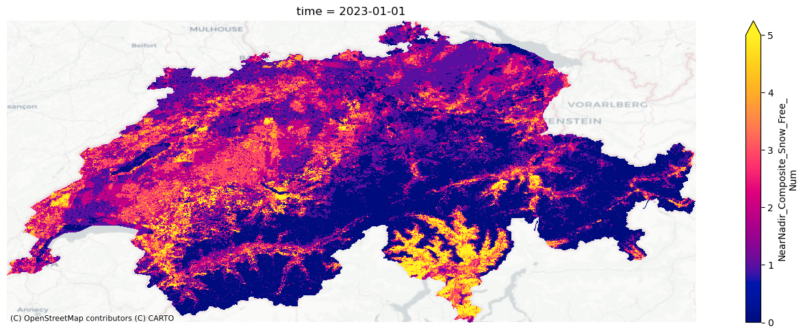
Number of Observations #
Black Marble removes poor quality observations, such as pixels covered by clouds. To determine the number of observations used to generate nighttime light values for each pixel, we add _Num to the variable name.
cf_r = bm_raster(
    gdf,
    product_id="VNP46A3",
    date_range="2023-01-01",
    token=bearer,
    variable="NearNadir_Composite_Snow_Free_Num",
)
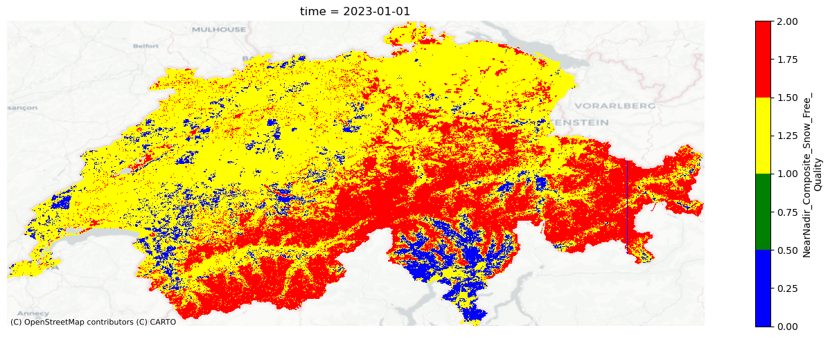
Quality #
For monthly and annual data, the quality values are:
0: Good-quality, The number of observations used for the composite is larger than 3
1: Poor-quality, The number of observations used for the composite is less than or equal to 3
2: Gap filled NTL based on historical data
255: Fill value
We can map quality by adding _Quality to the variable name.
quality_r = bm_raster(
    gdf,
    product_id="VNP46A3",
    date_range="2023-01-01",
    token=bearer,
    variable="NearNadir_Composite_Snow_Free_Quality",
)
Nighttime lights for good quality observations #
The quality_flag_rm parameter determines which pixels are set to NA based on the quality indicator. By default, only pixels with a value of 255 are filtered out. However, if we also want to remove poor quality pixels, we can adjust the quality_flag_rm parameter.
ntl_good_qual_r = bm_raster(
    gdf,
    product_id="VNP46A3",
    date_range="2023-01-01",
    token=bearer,
    variable="NearNadir_Composite_Snow_Free",
    quality_flag_rm=[1, 255],
)