SMOD Analyzer#
![]()

![]()
Introduction#
GHS-SMOD (Global Human Settlement Layer – Settlement Model Layer) provides valuable information on urbanization processes. The SMOD raster dataset, covering the period from 1975 to 2030 in 5-year intervals, offers estimated land use classifications for each 1 km × 1 km grid cell globally.
However, extracting the classified pixel information (such as Urban Center, Suburban, and Rural Cluster) from the SMOD dataset into the Areas of Interest (AOIs) for your project is not straightforward.
SMOD Analyzer, a Google-Colab-based Jupyter Notebook, provides an interactive interface to support this workflow. It enables national- and subnational-level data extraction by default with inline-visualization.
With the most minimal set-up, you only need to specify the ISO code of your target country. The notebook will then automatically generate: (1) National-level changes in urban and suburban–rural pixels over a 55-year period, and (2) Subnational-level (i.e., ADM-2 level) aggregations of each SMOD class for each subnational area and year, exported as an ESRI Shapefile—which is readily visualized on any GIS platform and can also be integrated with other related GIS datasets.
For those with knowledge of GIS and Python, this notebook serves as a good foundation for customizing workflows—for example, conducting SMOD analyses on user-defined AOIs such as specific urban areas.
Definition of SMOD classes:
- 30 Urban Centre
- 23 Dense Urban Cluster
- 22 Semi-Dense Urban Cluster
- 21 Suburban or Peri-urban
- 13 Rural Cluster
- 12 Low-density Rural
- 11 Very Low-density Rural
- 10 Rural Grid Cell (general)
- 0 No Population / Not classified / Water bodies
Example of reclassification (there is no definitive rule)
- Urban: 30, 23, 22
- Suburban: 21
- Rural: 13, 12, 11, 10
Usage#
Getting Started#
1. Prepare your Google Colab account#
As this notebook is optimized for the Google Colab (hereafter, Colab) environment, you must first create a Google account (if you don’t already have one) and access your Google Drive. If you have previously used Colab, you likely already have a “Colab Notebooks” directory. If not, please create one.
2. Download all SMOD-analyzer resources#
The must-haves for this notebook are:
Global ADM2 Boundary Shapefile (Preferably the latest World Bank Official ADM2 Shapefile (Not Public, Internal-use Only). Alternatively, World Health Organization ADM2 (Publicly Available))
Store these resources in a new directory (for example, ‘Analyzing GHS-SMOD’) following the directory structure below:
Analyzing GHS-SMOM/
│
├── data/
│   │
│   ├── shps/
│   │   ├──WHO_adm2/ (or WB official ADM2)
│   │   │   └──GLOBAL_ADM2.shp
│   │   └──Other AOI shapefile, if applicable
│   │
│   └── smod_row/
│       └──smod_1975.tif
│       └──smod_1980.tif
│       └── ...
│       └──smod_2030.tif
│
├── output/
│   └── Empty: Products will be stored here
│
├── SMOD_analyzer.ipynb
└── tools.py
3. Open the notebook in Google Colab#
Once you’ve opened the notebook in your Google Drive, start with the Initial Global Settings section. This section contains all the parameters you need to modify—unless you plan to implement more advanced or customized analyses.
(1) You first need to authorize the notebook to mount your Google Drive. Change the program_location if you store the notebook materials other than ‘Analyzing GHS-SMOD’.
from google.colab import drive
drive.mount('/content/drive')

program_location = '/content/drive/MyDrive/Colab Notebooks/Analyzing GHS-SMOD'
(2) Specify the 3-digit ISO of your target country. Here, ‘JPN’ (Japan) is specified as an example.
ISO = 'JPN'
(3) Find the most appropriate UTM for your target AOI, and specify it. For example,
NGA - WGS 84/UTM zone 31N (EPSG:26331)
IND - WGS 84/UTM zone 42N - 44N - 47N (EPSG:32642, EPSG:32644, EPSG:32647)
JPN - WGS 84/UTM zone 53N (EPSG:32653)
Here, ‘EPSG:32653’ for Japan is specified as an example.
UTM_crs = 'EPSG:32653'
(4) Finally, specify the unique ID for each ADM-2 boundary area (for WHO ADM2 data, it is ‘GUID’).
unique_ID = 'GUID'
4. Run all remaining sections#
Simply run all the remaining sections. The entire process may take some time to complete.
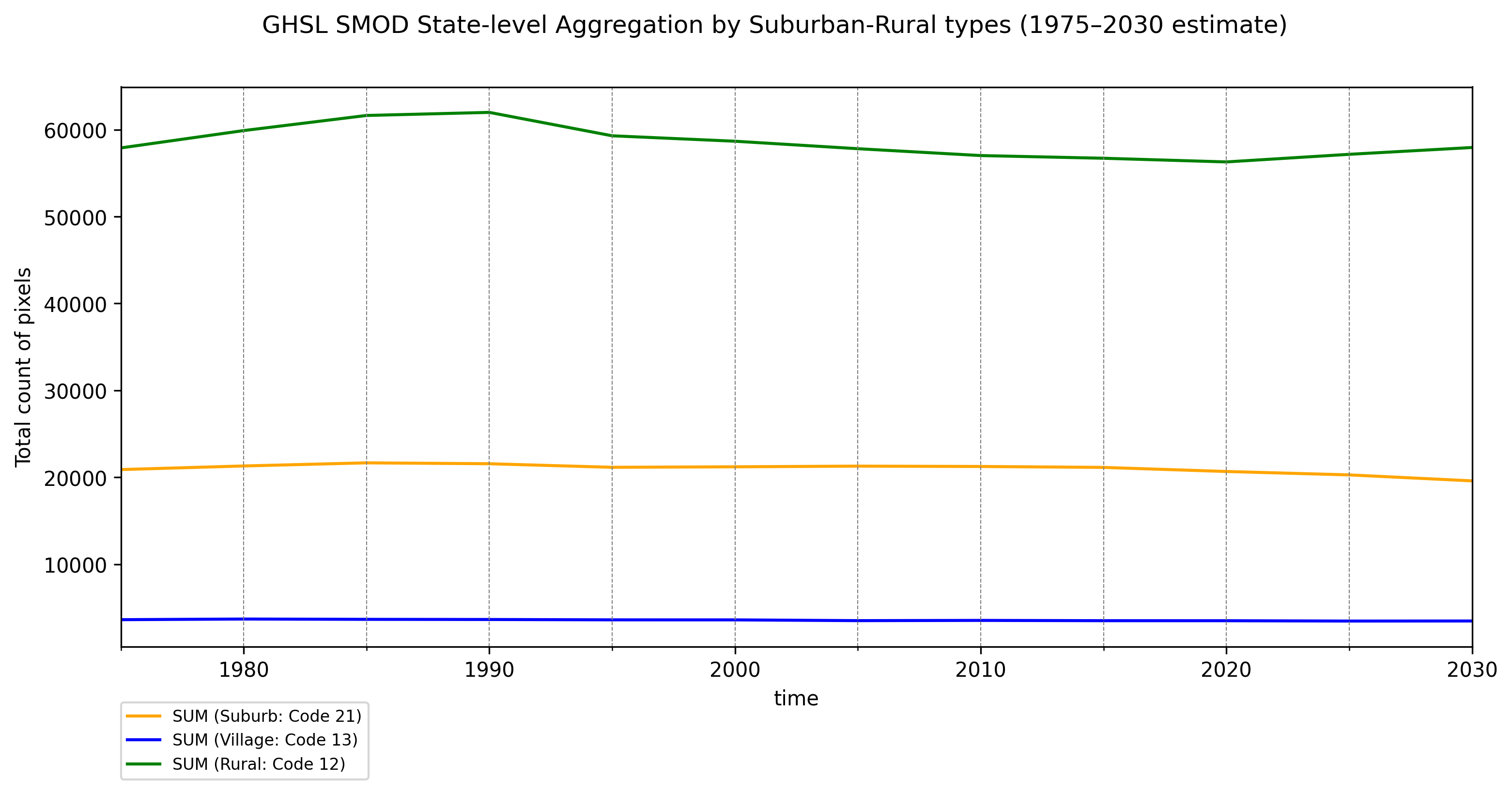
For the national-level SMOD analysis, you will obtain two graphs that illustrate trends in urbanization, suburbanization, and rural development (or decline):
Fig.1: Estimated urbanization trend in Japan
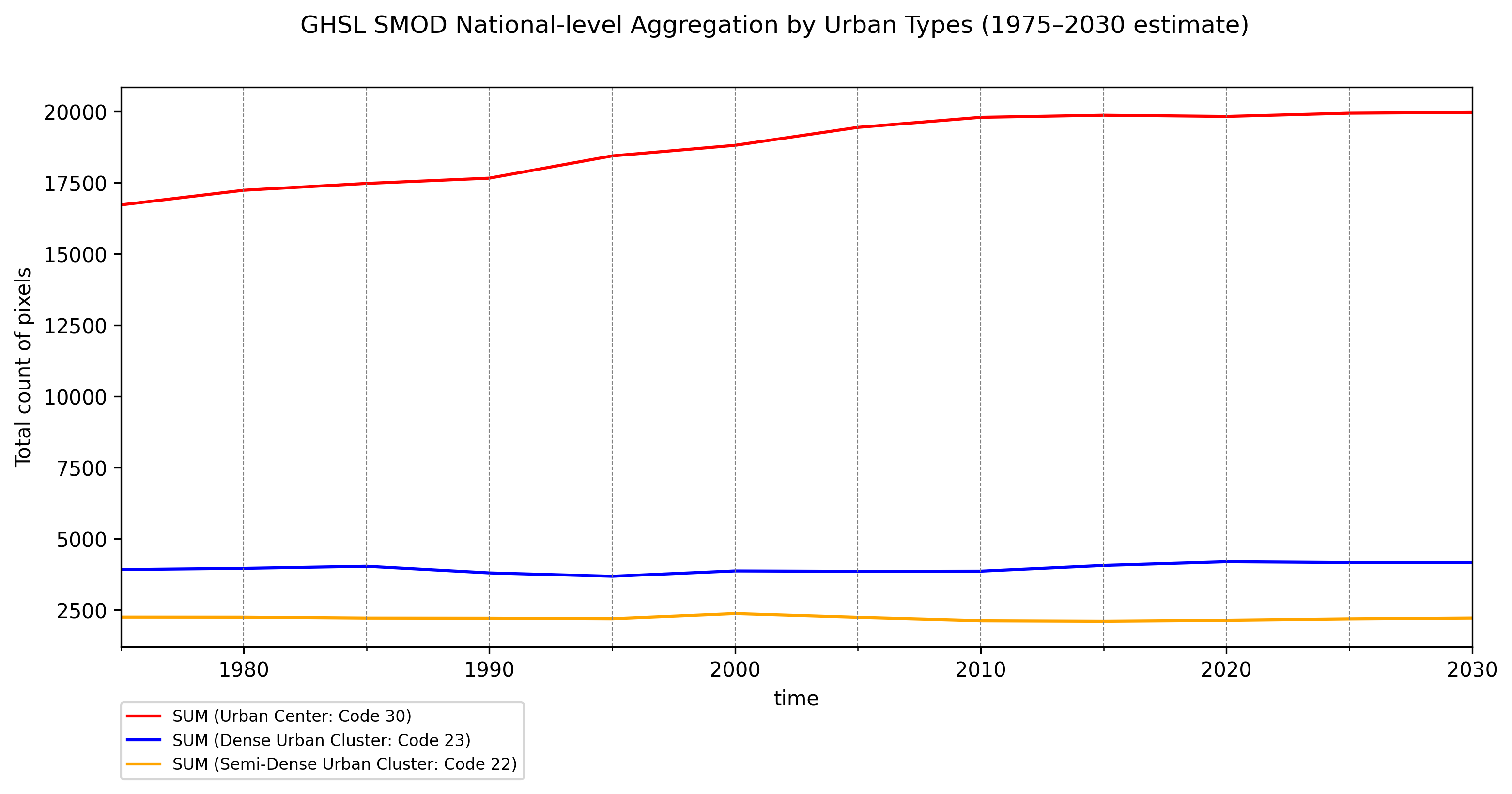
Fig.2: Estimated suburbanization and rural development trend in Japan
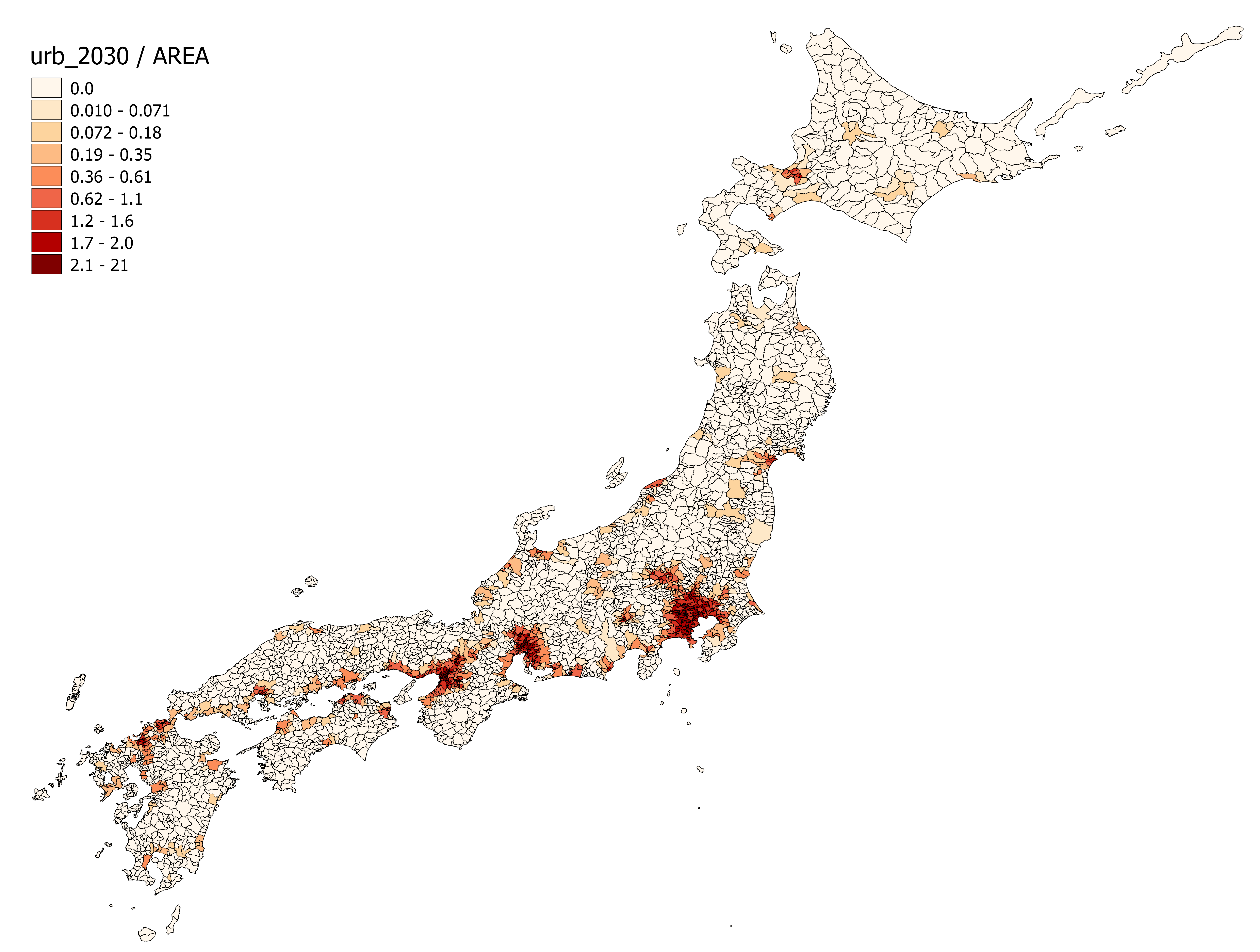
For the subnational (i.e., ADM-2 level) analysis, you will obtain a CSV file containing pixel counts for each SMOD class per ADM-2 area per year. (Note: the table may be very large if your target country has many ADM-2 areas.)
For spatial visualization, the same data—along with geometries—will also be exported as an ESRI Shapefile.
Fig.3: Estimated area-standardized Urban Cluster pixel counts in 2030 in Japan
Code of Conduct#
The SMOD_analyzer maintains a Code of Conduct to ensure an inclusive and respectful environment for everyone. Please adhere to it in all interactions within our community.
License#
The SMOD_analyzer is licensed under the Mozilla Public License. Remember to replace the license if necessary. If open source, choose an open source license.