S2S Haiti - Zonal statistics

Zonal statistics are run on the standardized H3 grid; the process is run on a country-by-country basis.

For the zonal statistics, each zonal statistic is run against the source dataset as a whole, then it is stratified by urban classification from the European Commission - GHS-SMOD. This creates an summary dataset that has the standard zonal stats columns (SUM, MEAN, MAX, MIN) as well as the same for urban areas (SUM_urban, MEAN_urban, MAX_urban, MIN_urban).

Show code cell source Hide code cell source

import sys, os, importlib, math, multiprocessing
import rasterio, geojson

import pandas as pd
import geopandas as gpd
import numpy as np

from h3 import h3
from tqdm import tqdm
from shapely.geometry import Polygon

sys.path.insert(0, "/home/wb411133/Code/gostrocks/src")
import GOSTRocks.rasterMisc as rMisc
import GOSTRocks.ntlMisc as ntl
import GOSTRocks.mapMisc as mapMisc
from GOSTRocks.misc import tPrint

sys.path.append("../src")
import h3_helper
import country_zonal

%load_ext autoreload
%autoreload 2

Show code cell source Hide code cell source

sel_iso3 = "HTI"
h3_level = 6

admin_bounds = "/home/public/Data/GLOBAL/ADMIN/ADMIN2/HighRes_20230328/shp/WB_GAD_ADM2.shp"
out_folder = f"/home/wb411133/projects/Space2Stats/{sel_iso3}"
if not os.path.exists(out_folder):
    os.makedirs(out_folder)
global_urban = "/home/public/Data/GLOBAL/GHSL/SMOD/GHS_SMOD_E2020_GLOBE_R2023A_54009_1000_V1_0.tif"

inA = gpd.read_file(admin_bounds)
selA = inA.loc[inA['ISO_A3'] == sel_iso3].copy()
selA['ID'] = selA.index #Create ID for indexing

inU = rasterio.open(global_urban)

# As a demo, we will process with nighttime lights layers
ntl_layers = ntl.aws_search_ntl()
ntl_file = ntl_layers[-1]

Generate zonal statistics at h3 based on urbanization levels

Show code cell source Hide code cell source

def get_per(x):
    try:
        return(x['SUM_urban']/x['SUM'] * 100)
    except:
        return(0)

Population

Show code cell source Hide code cell source

global_pop_layer = "/home/public/Data/GLOBAL/GHSL/Pop/GHS_POP_E2020_GLOBE_R2023A_54009_100_V1_0.tif"

zonalC = country_zonal.country_h3_zonal(sel_iso3, selA, "ID", h3_level, out_folder)
zonal_res_pop = zonalC.zonal_raster_urban(global_pop_layer, global_urban)

100%|██████████| 202/202 [00:01<00:00, 196.99it/s]

map_data_pop = zonal_res_pop.sort_values("SUM_urban").loc[:,['shape_id','SUM','SUM_urban']].copy()
map_data_pop = pd.merge(zonalC.h3_cells, map_data_pop, on='shape_id')
map_data_pop['per_urban'] = map_data_pop.apply(get_per, axis=1)
map_data_pop.sort_values('SUM')

	index	geometry	shape_id	index_right	ID	SUM	SUM_urban	per_urban
21	864c8a817ffffff	POLYGON ((-72.75291 20.09093, -72.77929 20.077...	864c8a817ffffff	36452	36452	-238.286994	0.0	-0.000000
73	864c8ad4fffffff	POLYGON ((-72.92188 20.09102, -72.94830 20.077...	864c8ad4fffffff	36452	36452	-229.921339	60.0	-26.095881
13	864c8a8a7ffffff	POLYGON ((-72.80921 20.09098, -72.83560 20.077...	864c8a8a7ffffff	36452	36452	-128.124768	413.0	-322.342048
602	8667258a7ffffff	POLYGON ((-72.03023 18.64439, -72.05657 18.630...	8667258a7ffffff	36503	36503	0.000000	0.0	0.000000
693	8667258afffffff	POLYGON ((-71.99667 18.60254, -72.02300 18.588...	8667258afffffff	36493	36493	0.000000	0.0	0.000000
...	...	...	...	...	...	...	...	...
679	866725c1fffffff	POLYGON ((-72.33478 18.60207, -72.36120 18.588...	866725c1fffffff	36488	36488	223787.948762	222807.0	99.561661
486	864c88687ffffff	POLYGON ((-72.20424 19.76281, -72.23052 19.749...	864c88687ffffff	36418	36418	233049.883958	231887.0	99.501015
528	866725c8fffffff	POLYGON ((-72.41407 18.55991, -72.44051 18.545...	866725c8fffffff	36487	36487	236411.146463	234849.0	99.339225
105	866725ce7ffffff	POLYGON ((-72.30118 18.56020, -72.32759 18.546...	866725ce7ffffff	36501	36501	320978.277533	319626.0	99.578701
186	866725cf7ffffff	POLYGON ((-72.35761 18.56006, -72.38404 18.546...	866725cf7ffffff	36501	36501	431109.360584	430148.0	99.777003

989 rows × 8 columns

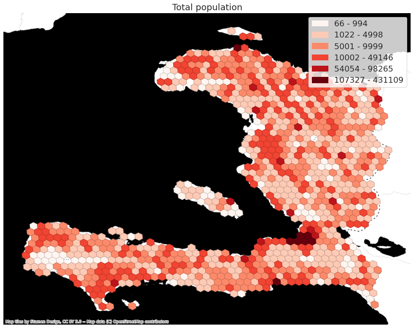
map_plt = mapMisc.static_map_vector(map_data_pop, "SUM", thresh=[50, 1000, 5000, 10000, 50000, 100000, 500000, 1500000], figsize=(15, 15))
map_plt.title("Total population")
map_plt.show()

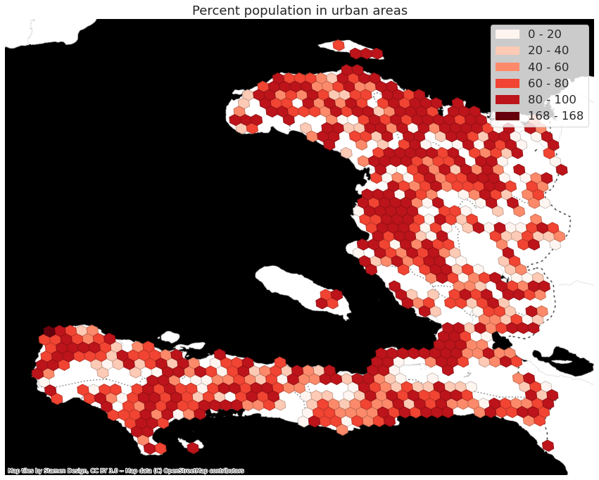
map_plt = mapMisc.static_map_vector(map_data_pop, "per_urban", thresh=[0, 20, 40, 60, 80, 100, 1000], figsize=(15,15))
map_plt.title("Percent population in urban areas")
map_plt.show()

Nighttime Lights

zonalC = country_zonal.country_h3_zonal(sel_iso3, selA, "ID", h3_level, out_folder)
zonal_res = zonalC.zonal_raster_urban(ntl_file, global_urban)

100%|██████████| 202/202 [00:01<00:00, 198.70it/s]

map_data = zonal_res.sort_values("SUM_urban").loc[:,['shape_id','SUM','SUM_urban']].copy()
map_data = pd.merge(zonalC.h3_cells, map_data, on='shape_id')
map_data['per_urban'] = map_data.apply(get_per, axis=1)
map_data.sort_values('SUM')

	index	geometry	shape_id	index_right	ID	SUM	SUM_urban	per_urban
339	866725157ffffff	POLYGON ((-71.99766 18.39270, -72.02401 18.378...	866725157ffffff	36490	36490	38.020000	0.0	0.000000
718	86672515fffffff	POLYGON ((-71.96406 18.35068, -71.99041 18.336...	86672515fffffff	36492	36492	38.529999	0.0	0.000000
98	86672514fffffff	POLYGON ((-71.90776 18.35075, -71.93409 18.336...	86672514fffffff	36492	36492	38.549999	0.0	0.000000
345	866725027ffffff	POLYGON ((-72.05399 18.39262, -72.08036 18.378...	866725027ffffff	36490	36490	38.550003	0.0	0.000000
168	8667250a7ffffff	POLYGON ((-72.18953 18.35026, -72.21594 18.336...	8667250a7ffffff	36476	36476	38.949997	0.0	0.000000
...	...	...	...	...	...	...	...	...
946	864c8b977ffffff	POLYGON ((-71.73426 19.59698, -71.76043 19.583...	864c8b977ffffff	36440	36440	359.739990	256.0	71.162508
186	866725cf7ffffff	POLYGON ((-72.35761 18.56006, -72.38404 18.546...	866725cf7ffffff	36501	36501	635.240051	554.0	87.211126
386	866725c0fffffff	POLYGON ((-72.27837 18.60219, -72.30477 18.588...	866725c0fffffff	36502	36502	740.360046	673.0	90.901718
105	866725ce7ffffff	POLYGON ((-72.30118 18.56020, -72.32759 18.546...	866725ce7ffffff	36501	36501	817.319946	750.0	91.763330
679	866725c1fffffff	POLYGON ((-72.33478 18.60207, -72.36120 18.588...	866725c1fffffff	36488	36488	1188.530029	1113.0	93.645089

989 rows × 8 columns

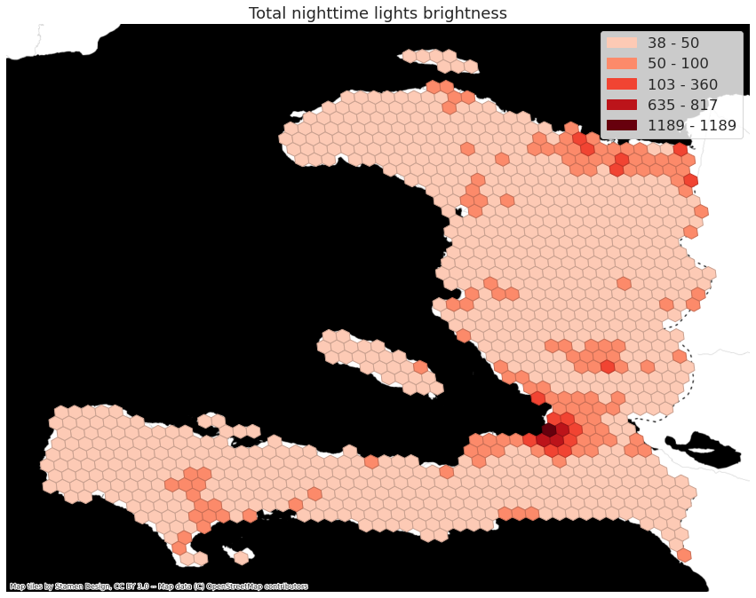
map_plt = mapMisc.static_map_vector(map_data, "SUM", thresh=[5,10,50,100,500,1000,7000], figsize=(15,15))
map_plt.title("Total nighttime lights brightness")
map_plt.show()

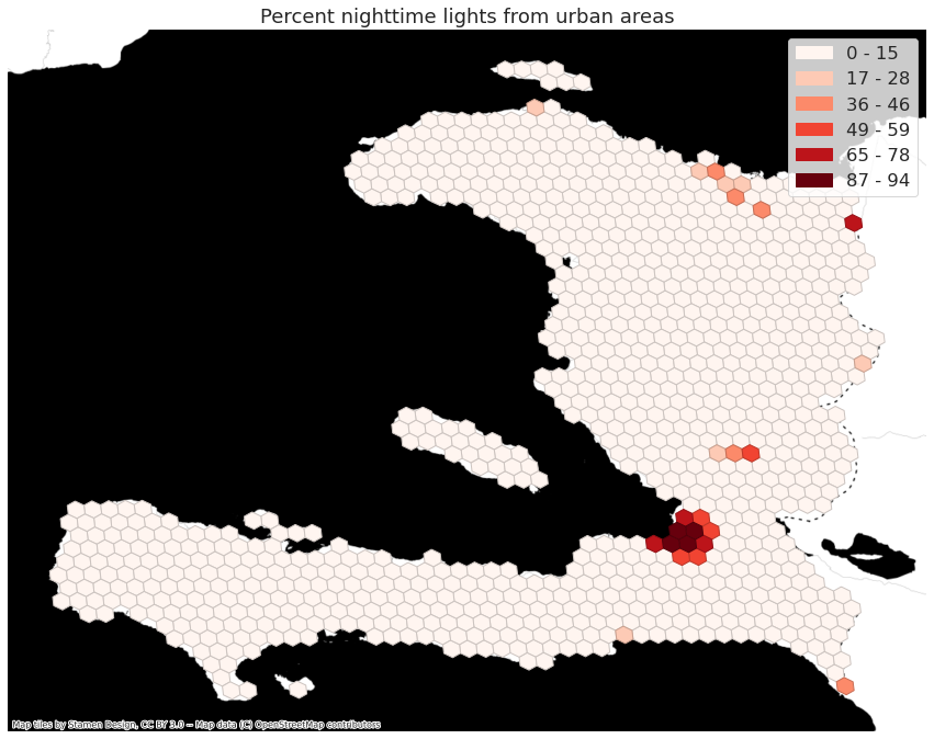
map_plt = mapMisc.static_map_vector(map_data, "per_urban", figsize=(15,15))
map_plt.title("Percent nighttime lights from urban areas")
map_plt.show()

Join h3 zonal results to admin boundaries

below we compare timing the administrative summaries with and without fractional intersections. While there is a difference between the two, the overall process is quite fast. As the is no computational limitation, we will rely on the fractional intersection as it is more accurate.

### These two cells are used to test the speed of joining with and without fractional intersection
%timeit cur_res = country_zonal.connect_polygons_h3_stats(selA, zonal_res, h3_level, "ID", True)

7.18 s ± 78 ms per loop (mean ± std. dev. of 7 runs, 1 loop each)

%timeit cur_res = country_zonal.connect_polygons_h3_stats(selA, zonal_res, h3_level, "ID", False)

6.76 s ± 17.2 ms per loop (mean ± std. dev. of 7 runs, 1 loop each)

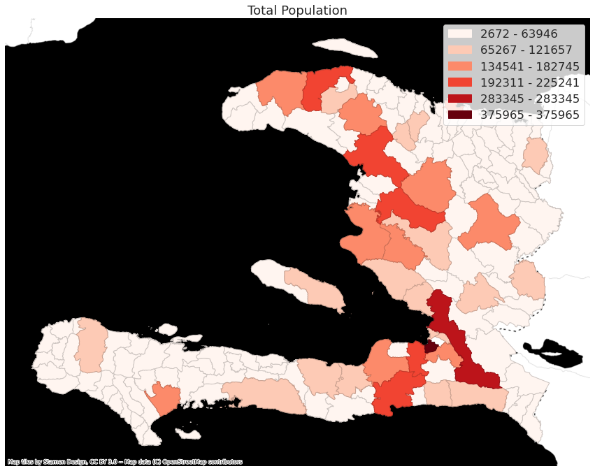
cur_res = country_zonal.connect_polygons_h3_stats(selA, zonal_res_pop, h3_level, "ID", True)

map_admin = pd.merge(selA, cur_res, left_on="ID", right_on='id')
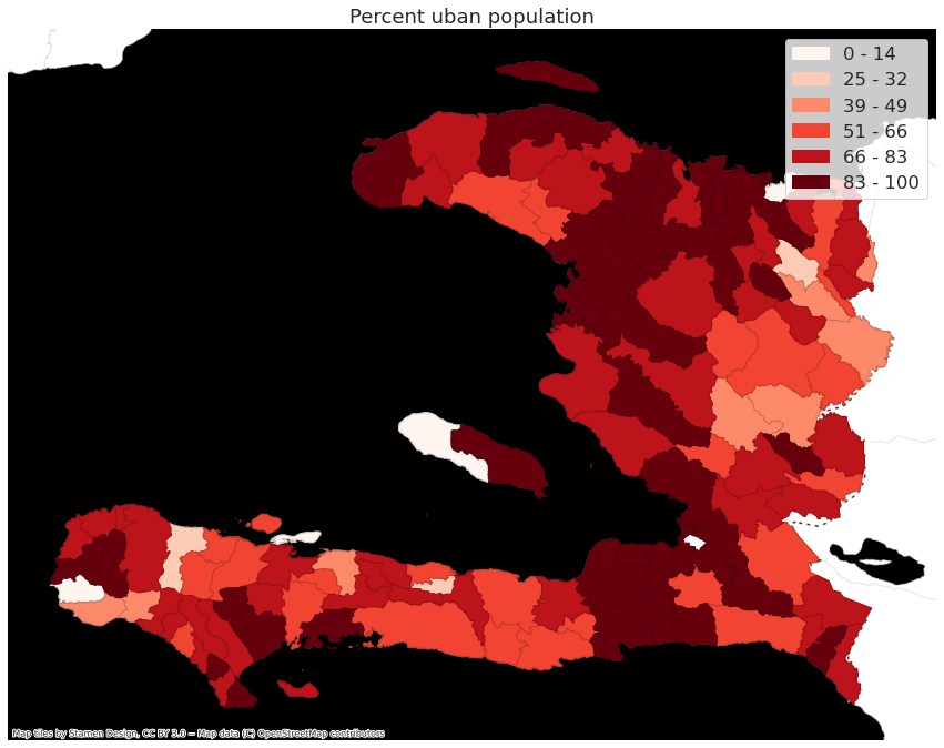
map_admin['per_urban'] = map_admin.apply(get_per, axis=1)

map_plt = mapMisc.static_map_vector(map_admin, "SUM", figsize=(15,15))
map_plt.title("Total Population")
map_plt.show()

map_plt = mapMisc.static_map_vector(map_admin, "per_urban", figsize=(15,15))
map_plt.title("Percent uban population")
map_plt.show()

Write output

map_data_pop.to_file(os.path.join(out_folder, "h3_urban_pop.geojson"), driver="GeoJSON")