S2S Kenya - Zonal statistics

Zonal statistics are run on the standardized H3 grid; the process is run on a country-by-country basis.

For the zonal statistics, each zonal statistic is run against the source dataset as a whole, then it is stratified by urban classification from the European Commission - GHS-SMOD. This creates an summary dataset that has the standard zonal stats columns (SUM, MEAN, MAX, MIN) as well as the same for urban areas (SUM_urban, MEAN_urban, MAX_urban, MIN_urban).

Show code cell source Hide code cell source

import sys, os, importlib, math, multiprocessing
import rasterio, geojson

import pandas as pd
import geopandas as gpd
import numpy as np

from h3 import h3
from tqdm import tqdm
from shapely.geometry import Polygon

sys.path.insert(0, "/home/wb411133/Code/gostrocks/src")
import GOSTRocks.rasterMisc as rMisc
import GOSTRocks.ntlMisc as ntl
import GOSTRocks.mapMisc as mapMisc
from GOSTRocks.misc import tPrint

sys.path.append("../src")
import h3_helper
import country_zonal

%load_ext autoreload
%autoreload 2

/home/wb411133/.conda/envs/ee/lib/python3.9/site-packages/geopandas/_compat.py:106: UserWarning: The Shapely GEOS version (3.9.1-CAPI-1.14.2) is incompatible with the GEOS version PyGEOS was compiled with (3.10.4-CAPI-1.16.2). Conversions between both will be slow.
  warnings.warn(

Show code cell source Hide code cell source

sel_iso3 = "KEN"
h3_level = 6

admin_bounds = "/home/public/Data/GLOBAL/ADMIN/ADMIN2/HighRes_20230328/shp/WB_GAD_ADM2.shp"
out_folder = f"/home/wb411133/projects/Space2Stats/{sel_iso3}"
if not os.path.exists(out_folder):
    os.makedirs(out_folder)
global_urban = "/home/public/Data/GLOBAL/GHSL/SMOD/GHS_SMOD_E2020_GLOBE_R2023A_54009_1000_V1_0.tif"

Show code cell source Hide code cell source

inA = gpd.read_file(admin_bounds)
selA = inA.loc[inA['ISO_A3'] == sel_iso3].copy()
selA['ID'] = selA.index #Create ID for indexing

inU = rasterio.open(global_urban)

Show code cell source Hide code cell source

# As a demo, we will begin with nighttime lights layers
ntl_layers = ntl.aws_search_ntl()
ntl_file = ntl_layers[-1]

Generate zonal statistics at h3 based on urbanization levels

Show code cell source Hide code cell source

def get_per(x):
    try:
        return(x['SUM_urban']/x['SUM'] * 100)
    except:
        return(0)

Population

Show code cell source Hide code cell source

global_pop_layer = "/home/public/Data/GLOBAL/GHSL/Pop/GHS_POP_E2020_GLOBE_R2023A_54009_100_V1_0.tif"
#popR = rasterio.open(global_pop_layer)
#popR.profile

zonalC = country_zonal.country_h3_zonal(sel_iso3, selA, "ID", h3_level, out_folder)
zonal_res_pop = zonalC.zonal_raster_urban(global_pop_layer, global_urban)

Generating h3 grid level 6: 100%|██████████| 365/365 [00:07<00:00, 50.52it/s]

(1, 11563, 7953)

zonal_res_pop

	SUM	MIN	MAX	MEAN	shape_id	SUM_urban	MIN_urban	MAX_urban	MEAN_urban
0	68.974775	0.0	17.155411	0.017668	867a413afffffff	0.0	0.0	0.0	0.000000
1	3.635393	0.0	3.635393	0.000946	867a740a7ffffff	0.0	0.0	0.0	0.000000
2	23259.264508	0.0	54.015900	5.928948	867a4c2afffffff	3698.0	0.0	1.0	0.942646
3	11.093490	0.0	2.705729	0.002883	867a4a9a7ffffff	0.0	0.0	0.0	0.000000
4	204.227029	0.0	59.439167	0.052950	867a43a87ffffff	0.0	0.0	0.0	0.000000
...	...	...	...	...	...	...	...	...	...
15246	1175.665880	0.0	39.080967	0.298468	867a4c99fffffff	126.0	0.0	1.0	0.031988
15247	92.193008	0.0	58.079727	0.024770	867a5bb0fffffff	0.0	0.0	0.0	0.000000
15248	53.785473	0.0	14.338305	0.014278	867a5d697ffffff	0.0	0.0	0.0	0.000000
15249	70.968876	0.0	19.066265	0.019243	867a5bcafffffff	0.0	0.0	0.0	0.000000
15250	7622.588723	0.0	61.932106	1.891461	867a69627ffffff	355.0	0.0	1.0	0.088089

15251 rows × 9 columns

map_data_pop = zonal_res_pop.sort_values("SUM_urban").loc[:,['shape_id','SUM','SUM_urban']].copy()
map_data_pop = pd.merge(zonalC.h3_cells, map_data_pop, on='shape_id')
map_data_pop['per_urban'] = map_data_pop.apply(get_per, axis=1)
map_data_pop.sort_values('SUM', ascending=False)

	shape_id	index_right	NAM_1	GAUL_2	NAM_2	geometry	SUM	SUM_urban	per_urban
0	867a42747ffffff	36824	Marsabit	0	Laisamis	POLYGON ((38.14369 1.55168, 38.15556 1.58313, ...	0.000000e+00	0.0	0.000000
2802	867a46c1fffffff	36689	Garissa	0	Balambala	POLYGON ((39.22998 0.19729, 39.24169 0.22906, ...	0.000000e+00	0.0	0.000000
7501	867a512d7ffffff	36894	Marsabit	0	North Horr	POLYGON ((38.44169 2.51242, 38.45345 2.54352, ...	0.000000e+00	0.0	0.000000
2806	866a58ae7ffffff	36955	Turkana	0	Turkana West	POLYGON ((34.84366 4.46588, 34.85599 4.49660, ...	0.000000e+00	0.0	0.000000
7494	867a66b17ffffff	36734	Tana River	0	Garsen	POLYGON ((39.17285 -2.98710, 39.18473 -2.95444...	0.000000e+00	0.0	0.000000
...	...	...	...	...	...	...	...	...	...
4746	867a6e417ffffff	36913	Nairobi	0	Roysambu	POLYGON ((36.93423 -1.21823, 36.94647 -1.18585...	4.574501e+05	455681.0	99.613269
9348	867a6e407ffffff	36913	Nairobi	0	Roysambu	POLYGON ((36.88711 -1.25555, 36.89936 -1.22315...	5.515042e+05	549574.0	99.650015
12245	867a6e55fffffff	36781	Nairobi	0	Kibra	POLYGON ((36.79280 -1.33023, 36.80507 -1.29781...	5.933135e+05	591558.0	99.704123
6380	867a6e437ffffff	36772	Nairobi	0	Kasarani	POLYGON ((36.94461 -1.27810, 36.95685 -1.24570...	7.745367e+05	772815.0	99.777711
9201	867a6e427ffffff	36839	Nairobi	0	Makadara	POLYGON ((36.89748 -1.31544, 36.90974 -1.28303...	1.188181e+06	1186359.0	99.846667

15251 rows × 9 columns

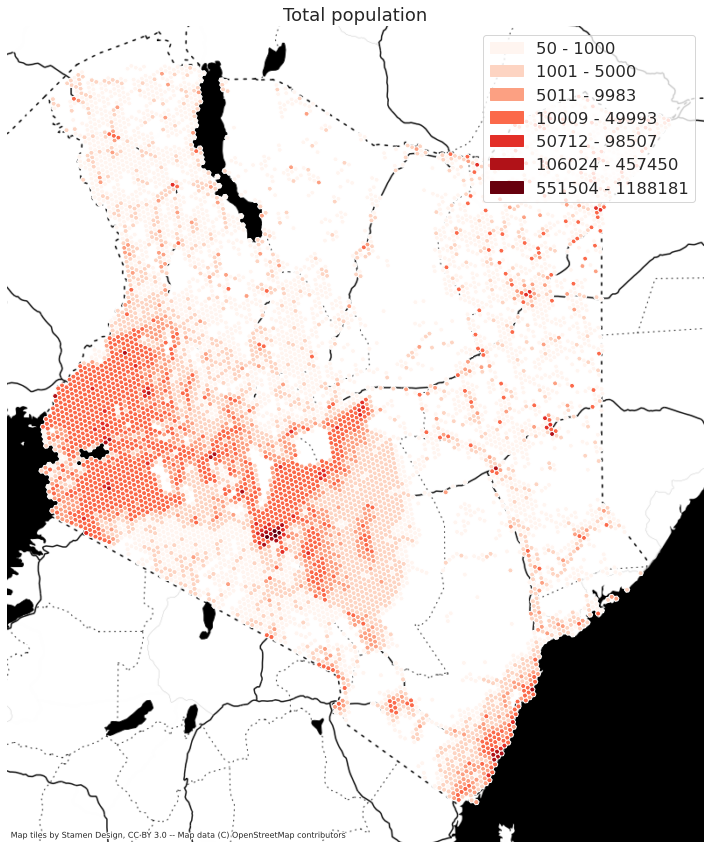
map_plt = mapMisc.static_map_vector(map_data_pop, "SUM", thresh=[50, 1000, 5000, 10000, 50000, 100000, 500000, 1500000], figsize=(15, 15))
map_plt.title("Total population")
map_plt.show()

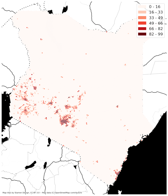
map_plt = mapMisc.static_map_vector(map_data_pop, "per_urban", thresh=[0, 20, 40, 60, 80, 100, 1000], figsize=(15,15))
map_plt.title("Percent population in urban areas")
map_plt.show()

Nighttime Lights

Show code cell source Hide code cell source

zonalC = country_zonal.country_h3_zonal(sel_iso3, selA, "ID", h3_level, out_folder)
zonal_res = zonalC.zonal_raster_urban(ntl_file, global_urban)

map_data = zonal_res.sort_values("SUM_urban").loc[:,['shape_id','SUM','SUM_urban']].copy()
map_data = pd.merge(zonalC.h3_cells, map_data, on='shape_id')
map_data['per_urban'] = map_data.apply(get_per, axis=1)
map_data.sort_values('SUM', ascending=False).head()

	shape_id	index_right	NAM_1	GAUL_2	NAM_2	geometry	SUM	SUM_urban	per_urban
6351	866a58a67ffffff	36955	Turkana	0	Turkana West	POLYGON ((34.92733 4.59296, 34.93965 4.62362, ...	36.120003	0.0	0.000000
8183	866a59b0fffffff	36953	Turkana	0	Turkana North	POLYGON ((35.87276 4.59425, 35.88490 4.62484, ...	37.129997	0.0	0.000000
1634	866a59857ffffff	36953	Turkana	0	Turkana North	POLYGON ((35.61105 4.59085, 35.62324 4.62146, ...	39.250000	0.0	0.000000
2795	866a58bafffffff	36955	Turkana	0	Turkana West	POLYGON ((34.66464 4.58921, 34.67700 4.61989, ...	39.839996	0.0	0.000000
12170	867ae185fffffff	36844	Mandera	0	Mandera North	POLYGON ((40.98292 3.56723, 40.99410 3.59766, ...	40.509998	0.0	0.000000
...	...	...	...	...	...	...	...	...	...
11618	867a6e42fffffff	36968	Nairobi	0	Westlands	POLYGON ((36.83997 -1.29288, 36.85223 -1.26047...	4407.709961	4147.0	94.085138
12431	867b59b2fffffff	36711	Mombasa	0	Changamwe	POLYGON ((39.63531 -4.06321, 39.64715 -4.03034...	4457.299805	3930.0	88.169972
579	867b59b27ffffff	36872	Mombasa	0	Mvita	POLYGON ((39.69284 -4.08543, 39.70467 -4.05255...	4545.560547	4409.0	96.995738
9201	867a6e427ffffff	36839	Nairobi	0	Makadara	POLYGON ((36.89748 -1.31544, 36.90974 -1.28303...	6022.190430	5929.0	98.452549
6380	867a6e437ffffff	36772	Nairobi	0	Kasarani	POLYGON ((36.94461 -1.27810, 36.95685 -1.24570...	6690.269531	6595.0	98.575999

15251 rows × 9 columns

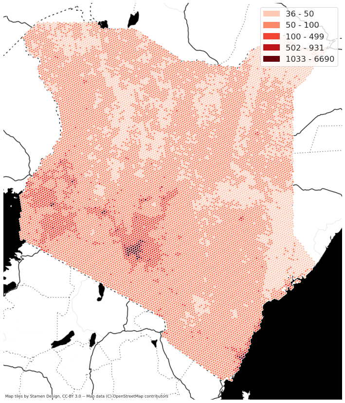
map_plt = mapMisc.static_map_vector(map_data, "SUM", thresh=[50,100,500,1000,7000], figsize=(15,15))
map_plt.title("Total Nighttime Brightness")
map_plt.show()

map_plt = mapMisc.static_map_vector(map_data, "per_urban", figsize=(15,15))
map_plt.title("Percent nighttime lights in urban areas")
map_plt.show()

Flood Depth

Show code cell source Hide code cell source

flood_depth = '/home/public/Data/GLOBAL/FLOOD_SSBN/v2_2019/Kenya/fluvial_undefended/FU_1in1000.tif'
zonalC = country_zonal.country_h3_zonal(sel_iso3, selA, "ID", h3_level, out_folder)
zonal_res = zonalC.zonal_raster_urban(flood_depth, global_urban, minVal=0, maxVal=10)

map_data = zonal_res.sort_values("SUM_urban").loc[:,['shape_id','SUM','SUM_urban']].copy()
map_data = pd.merge(zonalC.h3_cells, map_data, on='shape_id')
map_data['per_urban'] = map_data.apply(get_per, axis=1)
map_data.sort_values('SUM', ascending=False).head()

	shape_id	index_right	NAM_1	GAUL_2	NAM_2	geometry	SUM	SUM_urban	per_urban
4829	866a59a77ffffff	36953	Turkana	0	Turkana North	POLYGON ((35.99526 4.49305, 36.00739 4.52367, ...	13498.005859	0.0	0.000000
5171	866a59a57ffffff	36953	Turkana	0	Turkana North	POLYGON ((36.00521 4.43604, 36.01734 4.46668, ...	9973.853516	0.0	0.000000
5318	866a59b57ffffff	36953	Turkana	0	Turkana North	POLYGON ((35.92904 4.57214, 35.94117 4.60273, ...	9751.447266	0.0	0.000000
5993	867a5da77ffffff	36952	Turkana	0	Turkana East	POLYGON ((36.21001 2.04327, 36.22222 2.07472, ...	9321.406250	0.0	0.000000
199	867b5b0cfffffff	36734	Tana River	0	Garsen	POLYGON ((40.35870 -2.50227, 40.37030 -2.46985...	8719.301758	79.0	0.906036

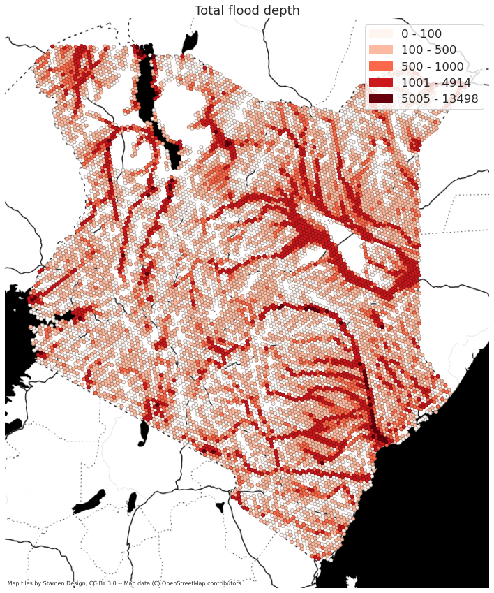
map_plt = mapMisc.static_map_vector(map_data, "SUM", thresh=[0,100,500,1000,5000,15000], figsize=(15,15))
map_plt.title("Total flood depth")
map_plt.show()

Show code cell source Hide code cell source

# Use flooding as mask for summing population
flood_r = rasterio.open(flood_depth)
flood_data = flood_r.read()
flood_data = ((flood_data > 0) * (flood_data < 100)).astype(int)
'''
flood_mask_file = os.path.join(out_folder, os.path.basename(flood_depth).replace(".tif", "_mask.tif"))
with rasterio.open(flood_mask_file, 'w', **flood_r.profile) as out_flood:
    out_flood.write(flood_data)
flood_mask = rasterio.open(flood_mask_file)
zonal_res = zonalC.zonal_raster_urban(global_pop_layer, flood_mask, minVal=0, urban_mask_val=[1])
'''
with rMisc.create_rasterio_inmemory(flood_r.profile, flood_data) as flood_mask:
    zonal_res_pop = zonalC.zonal_raster_urban(global_pop_layer, flood_mask, minVal=0, urban_mask_val=[1])

map_data_pop = zonal_res_pop.sort_values("SUM_urban").loc[:,['shape_id','SUM','SUM_urban']].copy()
map_data_pop = pd.merge(zonalC.h3_cells, map_data_pop, on='shape_id')
map_data_pop['per_urban'] = map_data_pop.apply(get_per, axis=1)
map_data_pop.sort_values('SUM', ascending=False).head()

	shape_id	index_right	NAM_1	GAUL_2	NAM_2	geometry	SUM	SUM_urban	per_urban
0	867a42747ffffff	36824	Marsabit	0	Laisamis	POLYGON ((38.14369 1.55168, 38.15556 1.58313, ...	-1	-1.0	100.0
10172	866a5914fffffff	36953	Turkana	0	Turkana North	POLYGON ((35.70693 4.34056, 35.71911 4.37125, ...	-1	-1.0	100.0
10160	867a7545fffffff	36729	Garissa	0	Fafi	POLYGON ((40.09253 -1.34859, 40.10414 -1.31645...	-1	-1.0	100.0
10161	867a74217ffffff	36747	Garissa	0	Ijara	POLYGON ((40.70511 -1.53392, 40.71660 -1.50179...	-1	-1.0	100.0
10162	867a61c77ffffff	36761	Kajiado	0	Kajiado South	POLYGON ((37.40516 -2.69114, 37.41739 -2.65841...	-1	-1.0	100.0

map_plt = mapMisc.static_map_vector(map_data_pop, "SUM", figsize=(15,15), thresh=[1,5000,10000,50000,100000,10000000],edgecolor="match")
map_plt.title("Population exposed to flood")
map_plt.show()

/home/wb411133/.conda/envs/ee/lib/python3.9/site-packages/contextily/tile.py:581: UserWarning: The inferred zoom level of 27 is not valid for the current tile provider (valid zooms: 0 - 20).
  warnings.warn(msg)

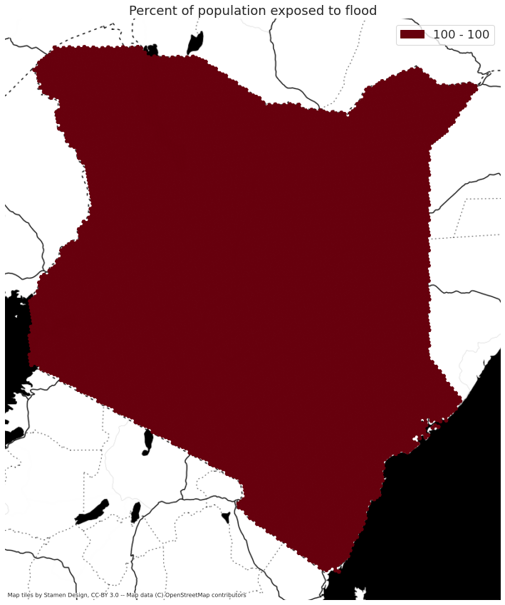
map_plt = mapMisc.static_map_vector(map_data_pop, "per_urban", figsize=(15,15), thresh=[1,25,50,70,90,100],edgecolor="match")
map_plt.title("Percent of population exposed to flood")
map_plt.show()

Join h3 zonal results to admin boundaries

below we compare timing the administrative summaries with and without fractional intersections. While there is a difference between the two, the overall process is quite fast. As the is no computational limitation, we will rely on the fractional intersection as it is more accurate.

### These two cells are used to test the speed of joining with and without
# %timeit cur_res = country_zonal.connect_polygons_h3_stats(selA, zonal_res, h3_level, "ID", True)

20.6 s ± 62.7 ms per loop (mean ± std. dev. of 7 runs, 1 loop each)

# %timeit cur_res = country_zonal.connect_polygons_h3_stats(selA, zonal_res, h3_level, "ID", False)

16.3 s ± 62.9 ms per loop (mean ± std. dev. of 7 runs, 1 loop each)

cur_res = country_zonal.connect_polygons_h3_stats(selA, zonal_res_pop, h3_level, "ID", True)

map_admin = pd.merge(selA, cur_res, left_on="ID", right_on='id')
map_admin['per_urban'] = map_admin.apply(get_per, axis=1)

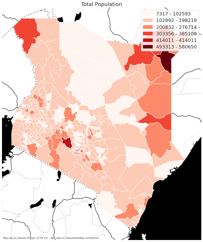
map_plt = mapMisc.static_map_vector(map_admin, "SUM", figsize=(15,15))
map_plt.title("Total Population")
map_plt.show()

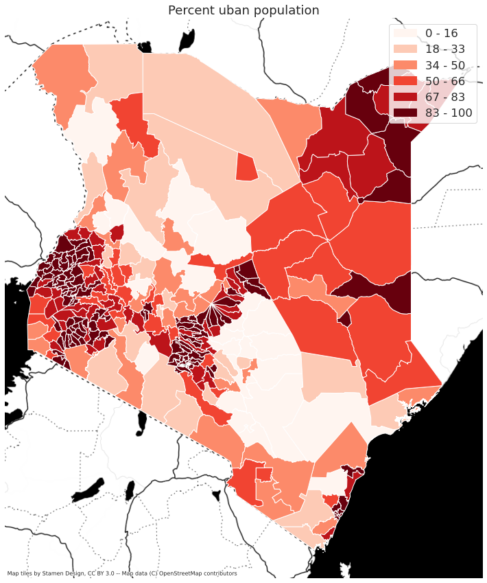
map_plt = mapMisc.static_map_vector(map_admin, "per_urban", figsize=(15,15))
map_plt.title("Percent uban population")
map_plt.show()

DEBUGGING

global_pop_layer = "/home/public/Data/GLOBAL/GHSL/Pop/GHS_POP_E2020_GLOBE_R2023A_54009_100_V1_0.tif"
popR = rasterio.open(global_pop_layer)
#popR.profile
rMisc.clipRaster(popR, zonalC.h3_cells, os.path.join(out_folder, os.path.basename(global_pop_layer)))

[array([[[-200., -200., -200., ..., -200., -200., -200.],
         [-200., -200., -200., ..., -200., -200., -200.],
         [-200., -200., -200., ..., -200., -200., -200.],
         ...,
         [-200., -200., -200., ..., -200., -200., -200.],
         [-200., -200., -200., ..., -200., -200., -200.],
         [-200., -200., -200., ..., -200., -200., -200.]]]),
 {'driver': 'GTiff',
  'dtype': 'float64',
  'nodata': -200.0,
  'width': 7913,
  'height': 11511,
  'count': 1,
  'crs': CRS.from_wkt('PROJCS["World_Mollweide",GEOGCS["WGS 84",DATUM["WGS_1984",SPHEROID["WGS 84",6378137,298.257223563,AUTHORITY["EPSG","7030"]],AUTHORITY["EPSG","6326"]],PRIMEM["Greenwich",0],UNIT["Degree",0.0174532925199433]],PROJECTION["Mollweide"],PARAMETER["central_meridian",0],PARAMETER["false_easting",0],PARAMETER["false_northing",0],UNIT["metre",1,AUTHORITY["EPSG","9001"]],AXIS["Easting",EAST],AXIS["Northing",NORTH]]'),
  'transform': Affine(100.0, 0.0, 3397700.0,
         0.0, -100.0, 574900.0)}]