Haiti Crop Productivity Analysis#
This notebook uses Enhanced Vegetation Index (EVI) from MODIS as a proxy for crop yield. EVI measures canopy greeness by analyzing spectral data through satellite imagery. EVI serves as a proxy for crop yield because it measures photosynthetic activity and green biomass, which strongly correlate with a crop’s potential productivity and final harvest output.
Methodology Summary#
Download imagery from MODIS for Haiti from 2012-2024.
Get Crop Mask data for Haiti from ESA
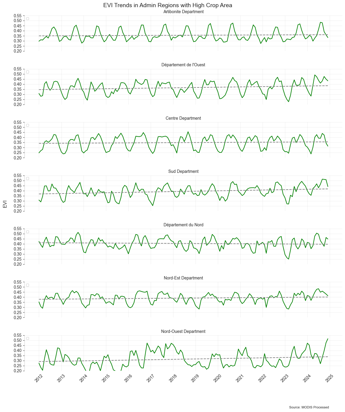
Estimate area of crop land in each admin region
Use 2021-2023 data as a baseline to identify growing season in Haiti
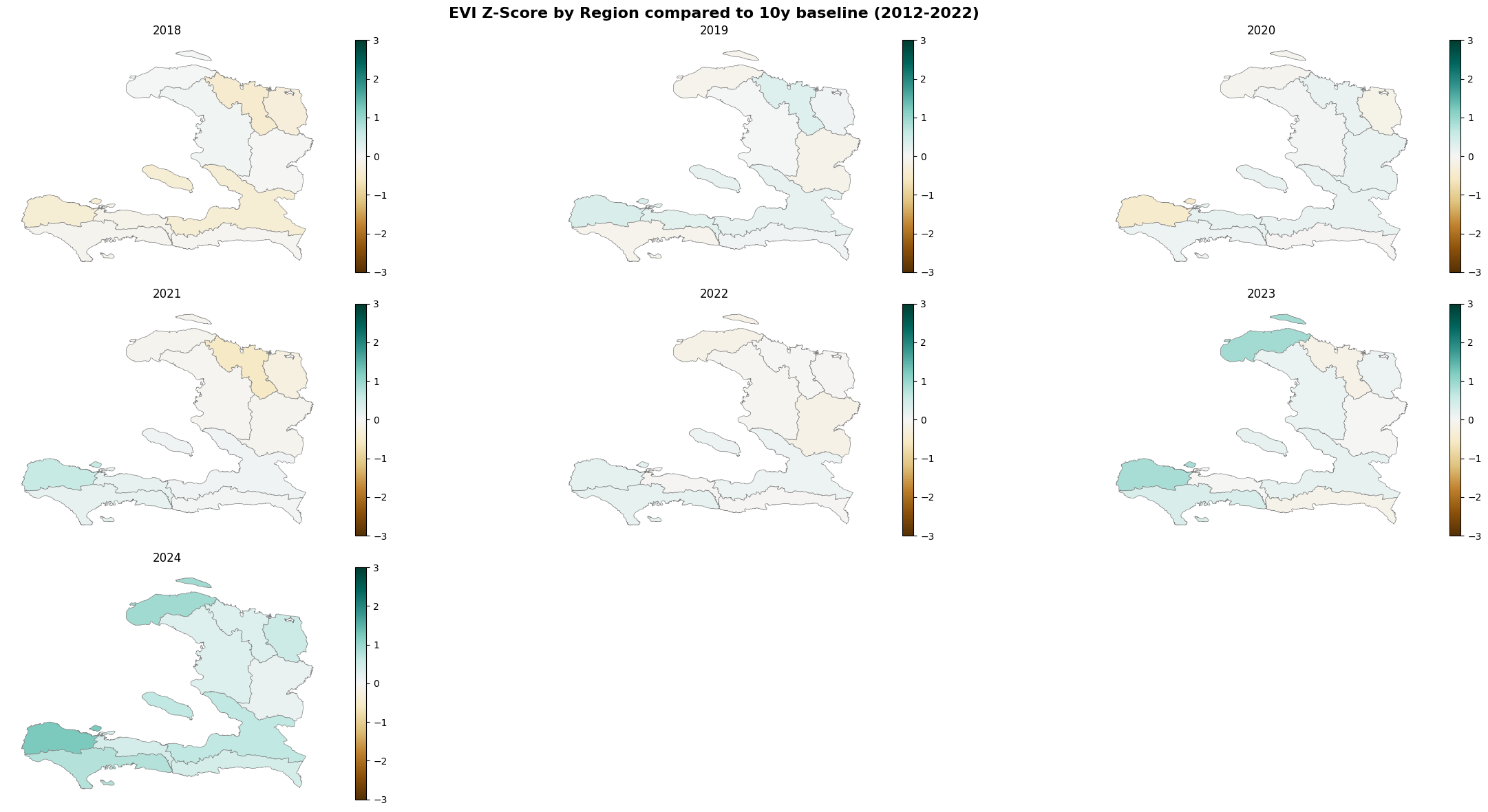
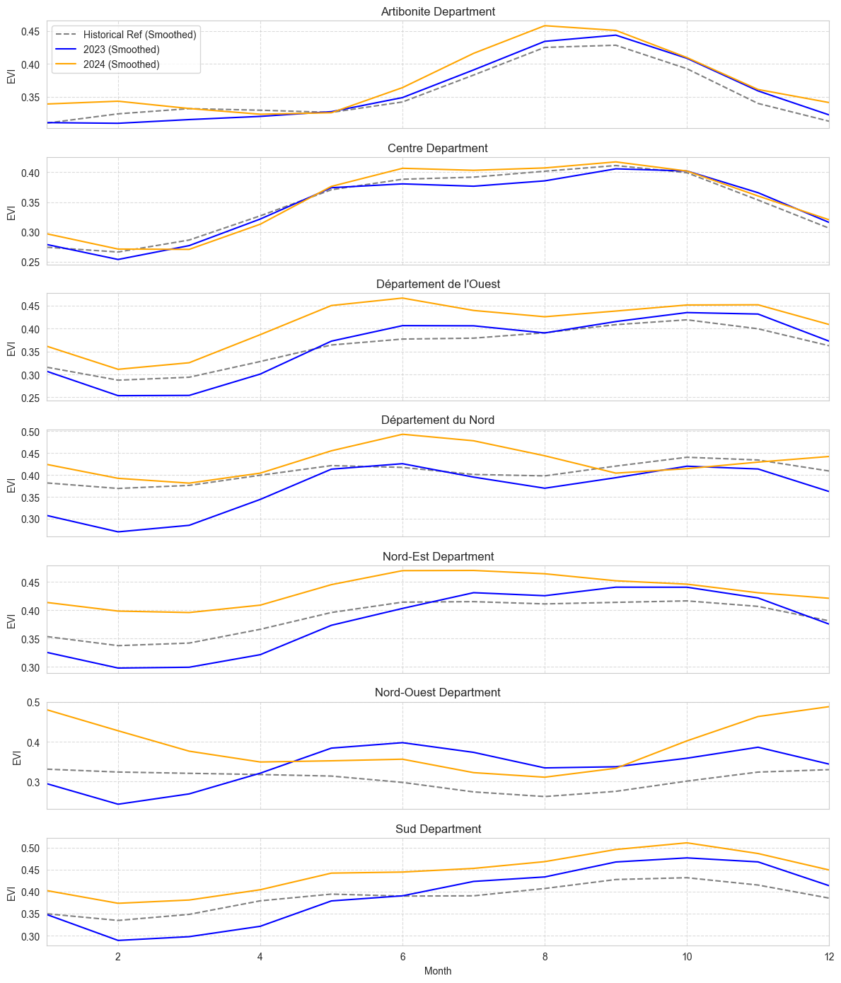
Use the growing season to track difference in EVI in 2024 compared to a 10 year average (2012-2022)
Plot trends in EVI over the last decade
MODIS#
We utilize Google Earth Engine to access the Enhanced Vegetation Index (EVI) band from the MODIS satellite. By combining data from Terra and Aqua, we obtain a map of EVI at 250 meters resolution every 16-days from 2012 to 2024.
The enhanced vegetation index (EVI) is an ‘optimized’ vegetation index designed to enhance the vegetation signal with improved vegetation monitoring through a de-coupling of the canopy background signal and a reduction in atmosphere influences.
We apply the necessary data masking steps:
Mask out bad quality data (shadows/clouds)
Mask out non-crop areas using the ESA crop layer.
The ESA Layers have the following information. We pick 40 for cropland. All other agricultural land that could be in other categories has not been considered for this analysis.
10: Tree cover
20: Shrubland
30: Grassland
40: Cropland
50: Built-up
60: Bare / sparse vegetation
70: Snow and ice
80: Permanent water bodies
90: Herbaceous wetland
95: Mangroves
100: Moss and lichen
Croparea Statistics#
| Region | Crop Area ha. | Crop Area Share (% of Country) | Crop Area Share (% of Region) | |
|---|---|---|---|---|
| 0 | Artibonite Department | 36,319 | 52.14% | 7.02% |
| 1 | Département de l'Ouest | 10,569 | 15.17% | 2.00% |
| 2 | Centre Department | 7,554 | 10.85% | 2.05% |
| 3 | Sud Department | 5,778 | 8.30% | 2.06% |
| 4 | Département du Nord | 4,086 | 5.87% | 1.82% |
| 5 | Nord-Est Department | 2,110 | 3.03% | 1.22% |
| 6 | Nord-Ouest Department | 1,644 | 2.36% | 0.74% |
| 7 | Département du Sud-Est | 1,349 | 1.94% | 0.63% |
| 8 | Département des Nippes | 219 | 0.31% | 0.17% |
| 9 | Département de la Grande-Anse | 23 | 0.03% | 0.01% |
Crop Seasonality#
Using this time series dataset of EVI images, we apply several pre-processing steps to extract critical phenological parameters: start of season (SOS), middle of season (MOS), end of season (EOS), length of season (LOS), etc. This workflow is heavily inspired by the TIMESAT software, although in this implementation we use the Phenolopy open-source package.
Pre-processing steps
Remove outliers from dataset on per-pixel basis using median method: outlier if median from a moving window < or > standard deviation of time-series times 2.
Interpolate missing values linearly
Smooth data on per-pixel basis (using Savitsky Golay filter, window length of 3, and polyorder of 1)
Phenology Process
We then extract crop seasonality metrics using the seasonal amplitude method from the phenolopy package.
The chart below shows the result of this process for a single crop pixel. The green dots represent the raw EVI values, the black line represents the processed EVI values, and the red dotted lines represent season parameters extracted for that pixel: start of season, peak of season, and end of season.
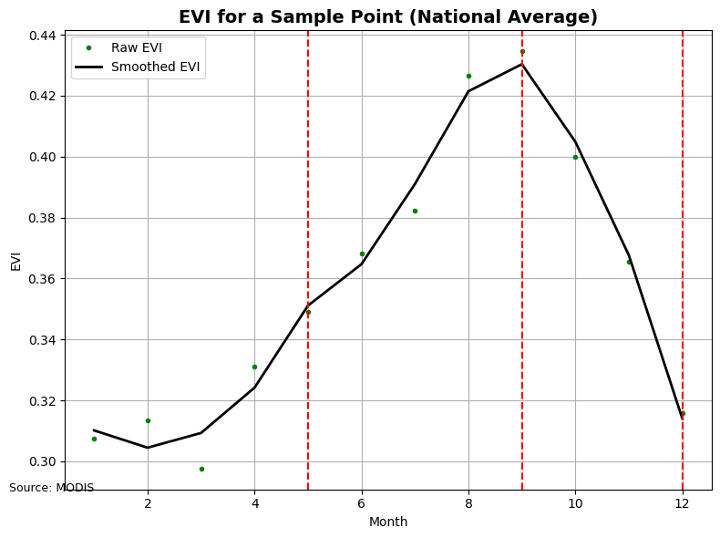
Based on the phenology process, we identified the seasonality to start in August and end in December with the peak being in September. This can vary with geographic region and crop type as well, however, that has not been taken into consideration in this version.
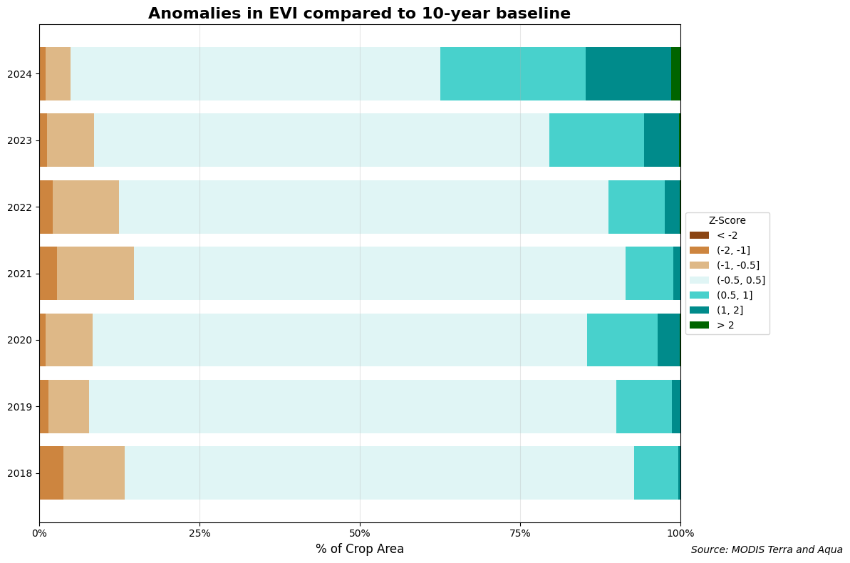
Anomalies in EVI#
Anomalies are calculated using z score values.
Where:
\(z\) is the z-score (standard score)
\(x\) is the individual median EVI value
\(\mu\) is the mean of the median EVI values
\(\sigma\) is the standard deviation of the median EVI values
The higher the variation the greater the anomaly i.e., if the value is -1 then the EVI for that time period is far lesser than the normal and vice versa.
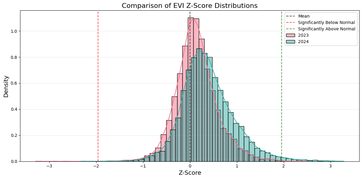
The Z scores are calculated for 2023 and 2024 compared to a historic 10 year average. They are then displayed as a histogram, a map and an aggregated map.
Statistical Summary:
--------------------------------------------------------------------------------
File                                           Mean     Median        Std     -1.96%     +1.96%
--------------------------------------------------------------------------------
2023                                          0.139      0.109      0.451        0.0        0.1
2024                                          0.390      0.329      0.561        0.0        1.3
--------------------------------------------------------------------------------
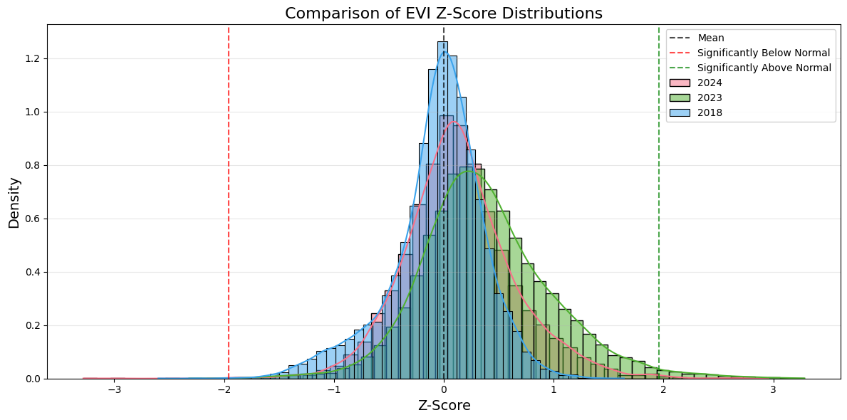
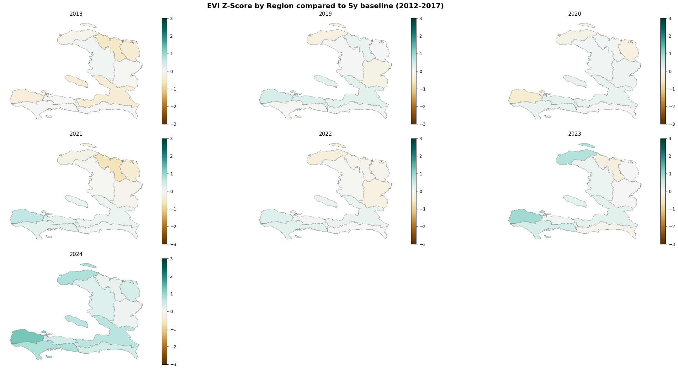
Calculating Z score compared to a baseline of 5 years from 2012-2017
Statistical Summary:
--------------------------------------------------------------------------------
File                                           Mean     Median        Std     -1.96%     +1.96%
--------------------------------------------------------------------------------
2024                                          0.139      0.110      0.513        0.1        0.2
2023                                          0.390      0.330      0.610        0.0        1.6
2018                                         -0.056     -0.008      0.431        0.1        0.0
--------------------------------------------------------------------------------
Interactive Map showing EVI anomalies
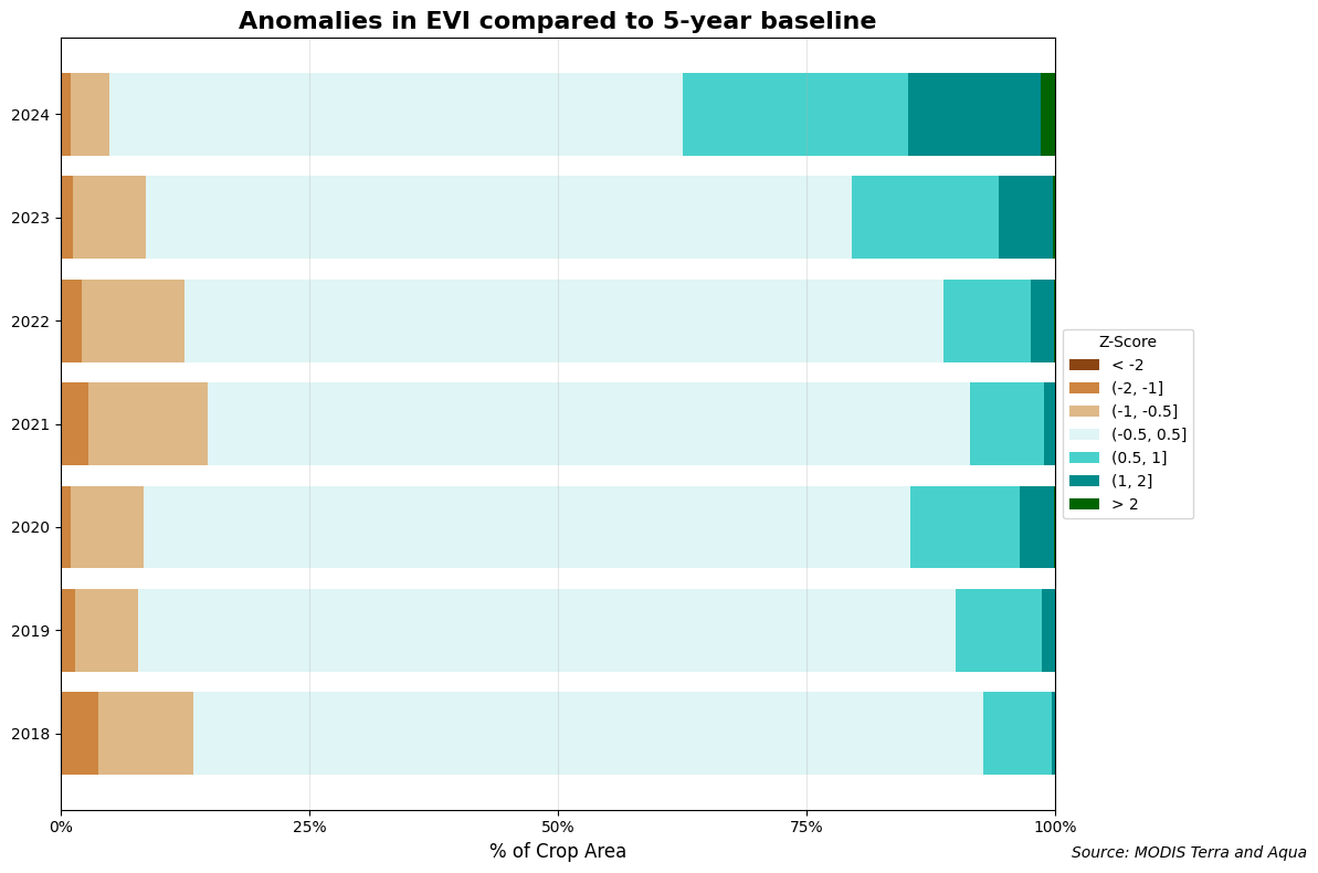
Mapping Z score compared to a 5 year baseline (2012-2017)
C:\Users\wb588851\AppData\Local\Temp\ipykernel_448\3575873206.py:43: UserWarning: No artists with labels found to put in legend.  Note that artists whose label start with an underscore are ignored when legend() is called with no argument.
  ax.legend(loc='upper left', fontsize=8)
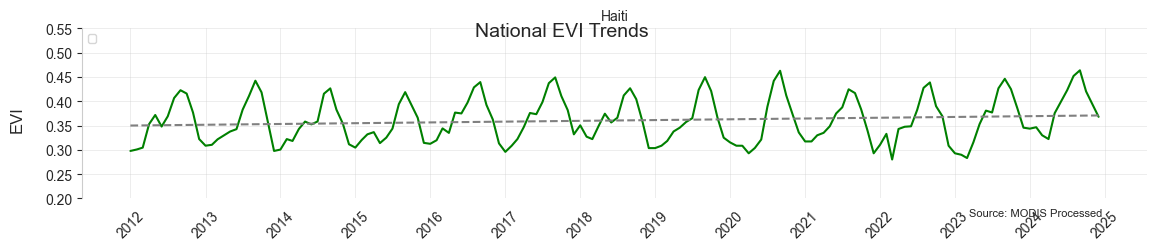
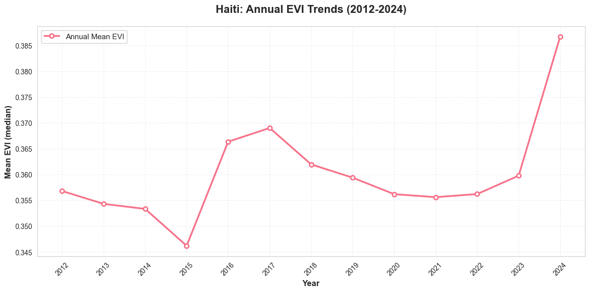
There is an increasing trend in EVI in Haiti since 2012. There were a few dips in 2021 and 2022 and there was recovery soon after.
C:\Users\wb588851\AppData\Local\Temp\ipykernel_448\3575873206.py:43: UserWarning: No artists with labels found to put in legend.  Note that artists whose label start with an underscore are ignored when legend() is called with no argument.
  ax.legend(loc='upper left', fontsize=8)
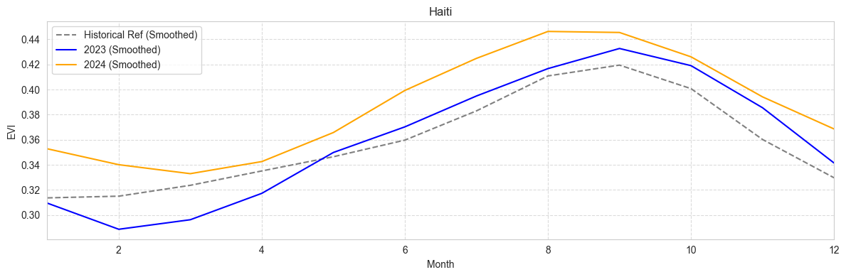
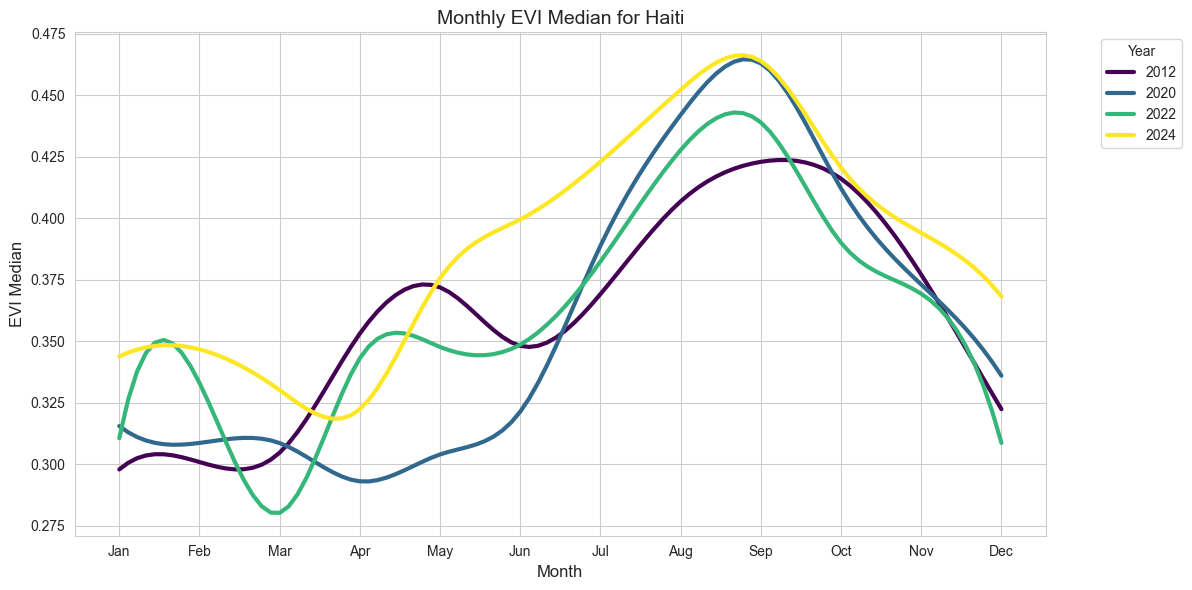
2024 was a better year for crop yield compared to the historic average. Although 2023 had a lower values in the beginning, the growing season saw greater crop yield.
Calculating Z-Score Anomalies in EVI for Detecting No-Planting Pixels#
The second part of the analysis aims to detect no-planting pixels using z-score anomalies in EVI and to calculate the extent of these areas within each Admin1 boundary. The methodology includes the following steps:
Calculating Z-Score Anomalies for EVI:
For each pixel, the z-score is calculated based on the EVI values for 2023 and 2024 relative to the mean and standard deviation of the previous ten years (2012-2022). This standardizes the data and highlights deviations from normal productivity.
Pixels with z-scores below a certain threshold (in this case, below 2 negative standard deviations) are classified as “no-planting” pixels, indicating a significant reduction in vegetation cover.
Summing No-Planting Pixel Areas:
The areas of no-planting pixels are calculated by multiplying the number of detected pixels by the pixel area (in hectares).
These areas are aggregated per Admin1 boundary to estimate the total extent of no-planting regions.
Calculating Total Cropland and Percent No-Planting Areas:
The total cropland area for each Admin1 region is calculated and the percentage of no-planting areas is calculated by against the total cropland area within each Admin1 boundary.
noplanting[(noplanting['threshold'] == -2)&(noplanting['no_planting_area_km2'] > 0)]
| year | threshold | admin_id | admin_name | total_area_km2 | no_planting_area_km2 | percentage_no_planting | |
|---|---|---|---|---|---|---|---|
| 220 | 2023 | -2.0 | 0 | Département de l'Ouest | 14409.63 | 0.19 | 0.0 |
There weren’t any significant no lanting zones detected using this methodology
Loaded data for years: [2018, 2019, 2020, 2021, 2022, 2023, 2024]
Loaded data for years: [2018, 2019, 2020, 2021, 2022, 2023, 2024]