Protest Classification Using LLM#
Objectives#
In this notebook, the objective is to use a Language Model (LLM) to classify each protest event in an ACLED dataset into predefined categories. Given this dataset which contains a note attribute providing detailed description about each protest event, leverage an LLM and example human labeled protest event to classify all protest evemts in the data so that we end up with dataset which will now have a predicted_category label.
Dataset#
In this task, we are using the same ACLED data being used for the rest of the conflict analysis. Howver, in addition, we are using an annotated dataset which provides classification of each protest event in the ACLED dataset. In this anotated dataset, whch we will refer to as training data, a team of experts working on Iran painstakingly labelled 224 instances of protest with two attributes as follows:
category. Each protest is classified into 6 categories.
Categories. ‘Livelihood (Prices, jobs and salaries)’, ‘Political/Security’, ‘Business and legal’, ‘Social’, ‘Public service delivery’, ‘Climate and environment’
Description This attribute provides a template defining core characteristics of each protest.
Overview of Approach#
 The Figure above provide an overview of the main steps we followed in this task.
Data Annotation. In order to use an LLM to perform this kind of classification accurately, the first step was to generate a training data by annotating a few hundred protest examples.
Zero-shot model evaluation and selection: To get a sense whether out of the box LLMs can accurately perfom this task as well as to pick which model to use, we tested a variety of open source and commercial LLMs to perform the classification task without any examples at all and found that OpenAI family of models gave superior performance. We therefore ended up using OpenAI models.
Assess few-shot classification and optimize LLM. At this stage, we profiled the perfomance of the selected OpenAI model to see how well it performs in a few-shot setting and also determine optimal number of parameter values such as number of examples to use and proper prompting strategy.
Classify the entire dataset Apply classification to the entire dataset using settings determined above.
Conduct quality assurance The final stage is to perform various sanity checks to make sure the classifications generated by the LLM are sensible, consistent with what happened on the ground.
More details about each of thes steps are provided in the respective section.
Global variables#
1. Preprocess Data and Explore the Labeled Dataset#
1.1 Explore the Labeled Protest Data#
In machine learning (ML) and working with LLMs, the labeled data containing examples of the six protest categories is referred to as training data. This data is used to train or guide the ML/LLM model in distinguishing between the different categories.
Our dataset includes a total of 224 examples. Understanding the distribution of this training data is crucial, as it directly impacts the performance of the ML model.
Show code cell source
pretty_print_value_counts(df_prot, "category",
title="Distribution of Protest Classes", line_length=60)
============================================================
              Distribution of Protest Classes
============================================================
| Category | Count | Percent | Cum. Percent |
|---|---|---|---|
| Livelihood (Prices, jobs and salaries) | 64 | 28.57% | 28.57% |
| Political/Security | 56 | 25.00% | 53.57% |
| Business and legal | 42 | 18.75% | 72.32% |
| Social | 26 | 11.61% | 83.93% |
| Public service delivery | 25 | 11.16% | 95.09% |
| Climate and environment | 11 | 4.91% | 100.00% |
2. Zero-shot Classification Performance#
What is zero-shot classification#
To select the best LLM or BERT-based model for our task, we first assess each model’s ability to classify text “out of the box,” without fine-tuning or examples. This zero-shot classification evaluation helps us gauge whether a model has the inherent capability to accurately categorize text in our dataset. Strong zero-shot performance indicates a model’s suitability and potential for further fine-tuning, allowing us to confidently narrow down our options before investing in training.
Measuring model performance#
We will use macro-precision, macro-recall and accuracy as our metrics for measuring model perfomance.
Accuracy:
Definition: Accuracy is the percentage of correct predictions made by the model out of all predictions.
Formula:
$\( \text{Accuracy} = \frac{\text{Number of Correct Predictions}}{\text{Total Predictions}} \times 100 \)$Explanation: If a model’s accuracy is 90%, it means the model correctly classified 90 out of every 100 items in the dataset. Accuracy is a helpful indicator of overall performance but might not give the full picture when dealing with multiple categories or unbalanced data (where some categories are much larger than others).
Precision:
Definition: Precision is the measure of how often the model’s predictions for a certain class are correct out of all the times it predicted that class.
Formula:
$\( \text{Precision} = \frac{\text{True Positives}}{\text{True Positives} + \text{False Positives}} \)$Explanation: Think of precision as answering the question, “When the model says something is in a particular category, how often is it right?” High precision means the model doesn’t make many false claims for a class. For example, if precision for the “positive” category is 80%, then out of all items the model labeled “positive,” 80% were truly positive. Precision is especially useful when we want to avoid falsely predicting a category.
Recall:
Definition: Recall is the measure of how well the model captures all items of a certain class out of the actual occurrences of that class in the dataset.
Formula:
$\( \text{Recall} = \frac{\text{True Positives}}{\text{True Positives} + \text{False Negatives}} \)$Explanation: Recall answers the question, “How many of the actual items in a class did the model successfully identify?” High recall means the model is good at finding most instances of a particular category. For example, if recall for “positive” is 85%, the model correctly labeled 85% of all truly positive items as “positive.” Recall is particularly important when we want to make sure we capture as many true items in a category as possible, even if we occasionally include incorrect ones.
When these metrics are averaged across multiple categories (like the six classes you have), they are referred to as macro precision and macro recall, ensuring all categories are given equal importance in the evaluation.
Comparing models#
We begin by comparing BERT, OpenAI’s GPT, and Llama3 models for text classification to assess each model’s strengths and find the best option for our needs. BERT represents a unique approach, focusing specifically on text classification, so we want to see if it achieves higher accuracy compared to the broader language models. Testing Llama3, an open-source model, lets us explore whether it can match or exceed the performance of proprietary models like GPT, providing us with a potentially powerful, cost-effective option.
For OpenAI’s GPT, we try to versions, GPT-4o and GPT-4o-mini. We are trying the older GPT-4-Turbo because it may offer similar perfomance while being cheaper and faster to run.
2.1 Show model performance#
Show code cell source
# ==============================
# PRINT OUT RESULTS
# ==============================
print(f"BERT Zero-shot Evaluation:\n  Accuracy: {bert_accuracy * 100:.2f}%\n  Macro Precision: {bert_macro_precision * 100:.2f}%\n  Macro Recall: {bert_macro_recall * 100:.2f}%\n")
print(f"LLaMA-3 Zero-shot Evaluation:\n  Accuracy: {llama_accuracy * 100:.2f}%\n  Macro Precision: {llama_macro_precision * 100:.2f}%\n  Macro Recall: {llama_macro_recall * 100:.2f}%\n")

# Display results with running times
print(f"GPT-4o Evaluation:\n  Accuracy: {gpt4_accuracy * 100:.2f}%\n  Macro Precision: {gpt4_macro_precision * 100:.2f}%\n  Macro Recall: {gpt4_macro_recall * 100:.2f}%\n  Runtime: {gpt4_runtime:.2f} seconds\n")
print(f"GPT-4o-min Evaluation:\n  Accuracy: {gpt4_min_accuracy * 100:.2f}%\n  Macro Precision: {gpt4_min_macro_precision * 100:.2f}%\n  Macro Recall: {gpt4_min_macro_recall * 100:.2f}%\n  Runtime: {gpt4_min_runtime:.2f} seconds\n")
print(f"GPT-4-turbo Evaluation:\n  Accuracy: {gpt4_turbo_accuracy * 100:.2f}%\n  Macro Precision: {gpt4_turbo_macro_precision * 100:.2f}%\n  Macro Recall: {gpt4_turbo_macro_recall * 100:.2f}%\n  Runtime: {gpt4_turbo_runtime:.2f} seconds\n")
BERT Zero-shot Evaluation:
  Accuracy: 8.93%
  Macro Precision: 2.42%
  Macro Recall: 15.03%

LLaMA-3 Zero-shot Evaluation:
  Accuracy: 9.38%
  Macro Precision: 3.08%
  Macro Recall: 10.04%

GPT-4o Evaluation:
  Accuracy: 82.59%
  Macro Precision: 60.53%
  Macro Recall: 54.77%
  Runtime: 158.39 seconds

GPT-4o-min Evaluation:
  Accuracy: 70.98%
  Macro Precision: 71.28%
  Macro Recall: 62.62%
  Runtime: 116.92 seconds

GPT-4-turbo Evaluation:
  Accuracy: 81.70%
  Macro Precision: 83.86%
  Macro Recall: 72.97%
  Runtime: 178.56 seconds
2.2 Analyze category misclassifications with a confusion matrix#
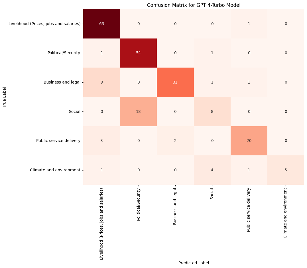
We selected the best-performing model under the zero-shot classification scenario and analyzed its performance in more detail. To do this, we used a confusion matrix to evaluate how well the model performed for each category in the training dataset.
The analysis revealed that the Social category had the highest number of misclassifications, with most notes being incorrectly labeled as Political/Security. Interestingly, the Political/Security category was rarely misclassified as Social. The second category with the highest misclassification rate was Climate and Environment. Let’s take a closer look at these misclassified notes.
These misclassifications can be further analyzed to determine whether there are inherent, indistinguishable similarities in how these categories are described in the dataset. A spreadsheet,
social-misclassifications.csv, has been saved to facilitate this inspection by individuals who are highly familiar with the dataset.
Show code cell source
# Generate the confusion matrix
conf_matrix = confusion_matrix(df_gpt4_turbo['category'], df_gpt4_turbo['predicted_category'], labels=CATEGORIES)

# Plot the confusion matrix with a red color palette
plt.figure(figsize=(10, 8))
sns.heatmap(conf_matrix, annot=True, fmt="d", cmap="Reds", xticklabels=categories, yticklabels=categories, cbar=False)
plt.xlabel("Predicted Label")
plt.ylabel("True Label")
plt.title("Confusion Matrix for GPT 4-Turbo Model")
plt.show()
3. Classify the Entire Dataset#
In the previous section, we evaluated the performance of several state-of-the-art LLMs and smaller language models (e.g., BERT) to understand how well they could classify the note into our predetermined six categories. Among these models, OpenAI’s GPT-4-turbo performed exceptionally well. Moving forward, we will use the GPT-4-turbo model to classify our entire target dataset, which includes the note and description columns providing detailed information about each protest. We will follow this process:
Use Few-Shot Learning to Improve GPT-4-turbo Performance#
In the earlier section, we assessed the performance of GPT-4-turbo and other models without providing them with any examples or additional training (zero-shot learning). In this scenario, GPT-4-turbo achieved an accuracy of 82%. However, the confusion matrix revealed significant variation in performance across categories. For instance, the precision for categories such as social was notably poor.
Now that we are classifying the entire dataset, we will leverage a technique called few-shot learning. This involves providing examples to the LLM and then asking it to classify data based on the patterns demonstrated in the examples. This approach almost always enhances the model’s performance.
Check Performance of GPT-4-turbo with Few-Shot Learning#
While we gained an initial understanding of how well GPT-4-turbo performed in the zero-shot classification scenario, it is important to quantify its performance when examples are provided. To achieve this, we will split our dataset of 212 training examples into a train set (e.g., 80% of the data) and a test set. We will then randomly select examples from the train set (e.g., 5, 10, 15 examples) to pass to the LLM and evaluate its performance. We will also revisit the confusion matrix to determine whether few-shot learning improves the model’s performance for categories such as social, which previously suffered from high misclassification rates.
Classify the entire dataset#
Once we determine the optimal number of examples to use, the most effective prompt strategy, and how well the few-shot example setting performs, we will apply the same prompt template, formatting, and settings to classify each protest. This will result in a new column, classification, being added to the dataset. Given that there are approximately 25,000 protest instances, this process typically takes around 2–3 hours, depending on the number of examples provided.
Perform Sanity Checks#
The steps above will give us confidence in how well the LLM performs. For instance, if the LLM achieves 90% accuracy, we can reasonably expect that approximately 90% of the classifications for the entire dataset will be correct. Beyond this, there are additional sanity checks we can perform to further validate the model’s classifications:
Compare the distribution of model classifications with the training data (212 examples):
While the distributions do not need to be identical, we expect them to be comparable. Significant discrepancies might indicate issues with the model’s classifications.Analyze the similarity of notes within a category versus across categories:
Intuitively, protest descriptions within a category (e.g., social) should exhibit greater semantic similarity (measured using techniques like cosine similarity) compared to descriptions from different categories. We will perform this analysis to confirm whether this pattern holds true.Verify classifications against real-world knowledge:
As previously demonstrated, we can cross-check classifications against actual historical data. For instance, if the LLM classifies a large number of protests as social in January 2024 but there is no record of such a spike, it may indicate misclassification by the LLM.
3.1 Assessing Classification Accuracy with Few-Shot Examples#
To evaluate GPT-4-turbo under few-shot learning, we will split our dataset of 212 training examples into a train set (e.g., 80%) and a test set. By providing varying numbers of examples (e.g., 5, 10, 15) from the train set, we aim to balance performance, running time, and cost while identifying the most effective prompting strategy. We will also revisit the confusion matrix to assess improvements in category-specific performance, such as social, which previously showed high misclassification rates.
3.1.1 Split the examples into training and test#
It’s important to note that this approach differs from the typical machine learning paradigm, where around 70-80% of the dataset is used for training and the remainder for evaluation. With LLMs like GPT-4-turbo, feeding too many examples slows down the process and significantly increases costs.
To evaluate how well the LLM performs under few-shot learning, it’s more practical to allocate a larger portion of the data for testing and a smaller portion for providing examples to the model. Therefore, we split the dataset into 40% for training and 60% for testing.
Examples for the model will be drawn from the 40% training portion, and the model’s performance will be evaluated on the 60% test portion. This strategy ensures we can thoroughly evaluate the model while keeping costs and runtime manageable.
Show code cell source
pretty_print_value_counts(train_df, "category",
title="Train-Distribution of Protest Classes", line_length=60)
============================================================
           Train-Distribution of Protest Classes
============================================================
| Category | Count | Percent | Cum. Percent |
|---|---|---|---|
| Livelihood (Prices, jobs and salaries) | 32 | 28.57% | 28.57% |
| Political/Security | 28 | 25.00% | 53.57% |
| Business and legal | 21 | 18.75% | 72.32% |
| Social | 13 | 11.61% | 83.93% |
| Public service delivery | 12 | 10.71% | 94.64% |
| Climate and environment | 6 | 5.36% | 100.00% |
Show code cell source
pretty_print_value_counts(test_df, "category",
title="Test-Distribution of Protest Classes", line_length=60)
============================================================
            Test-Distribution of Protest Classes
============================================================
| Category | Count | Percent | Cum. Percent |
|---|---|---|---|
| Livelihood (Prices, jobs and salaries) | 32 | 28.57% | 28.57% |
| Political/Security | 28 | 25.00% | 53.57% |
| Business and legal | 21 | 18.75% | 72.32% |
| Social | 13 | 11.61% | 83.93% |
| Public service delivery | 13 | 11.61% | 95.54% |
| Climate and environment | 5 | 4.46% | 100.00% |
3.1.2 . Prepare Examples#
For each example, we use three columns to provide information to the LLM: notes, description, and category. These columns must be formatted appropriately before being passed to the model.
We use a variable, NUM_EXAMPLES, to specify the number of examples per category to include. After experimenting with 5, 10, and 15 examples, we determined that 10 examples (which gives a total of 60 examples with 6 categories) strike the optimal balance. However, it’s important to note that some classes, such as climate, have only 11 examples available in the training dataset.
3.1.3 Prepare Prompt Template#
Experimenting with multiple templates is essential because the way information is presented to an LLM can significantly impact its performance. In this case, the template must ensure the model pays attention to all three columns: notes, description, and category. Additionally, the template should be designed to instruct the LLM to output only the classification, as models sometimes prepend additional text before the category or classification, which can lead to inconsistent results. By refining the template, we can maximize accuracy and ensure the outputs are structured correctly for downstreaming data processing and usage of the data.

Show code cell source
pretty_print_value_counts(test_df, "predicted_category",
title="Distribution- Predicted Categories in Test Set", line_length=60)
============================================================
       Distribution- Predicted Categories in Test Set
============================================================
| Category | Count | Percent | Cum. Percent |
|---|---|---|---|
| Livelihood (Prices, jobs and salaries) | 31 | 27.68% | 27.68% |
| Political/Security | 26 | 23.21% | 50.89% |
| Business and legal | 26 | 23.21% | 74.11% |
| Social | 13 | 11.61% | 85.71% |
| Public service delivery | 11 | 9.82% | 95.54% |
| Climate and environment | 5 | 4.46% | 100.00% |
Show code cell source
# Generate the confusion matrix
conf_matrix = confusion_matrix(test_df['category'], test_df['predicted_category'], labels=CATEGORIES)

# Plot the confusion matrix with a red color palette
plt.figure(figsize=(10, 8))
sns.heatmap(conf_matrix, annot=True, fmt="d", cmap="Reds", xticklabels=categories, yticklabels=categories, cbar=False)
plt.xlabel("Predicted Label")
plt.ylabel("True Label")
plt.title("Confusion Matrix for GPT 4-Turbo Model")
plt.show()

3.2 Classify All Documents#
We are now ready to classify all the documents in the dataset using the previously defined prompt template and example formatting strategy. This approach has achieved approximately 90% accuracy and precision for 112 test examples, utilizing 10 examples per category for a total of 60 examples.
# ========================================
# LOAD THE DATA AND PERFOM CLASSIFICATION
# ========================================
df_all = pd.read_csv(FILE_PROTESTS)
df_all.drop(columns=["Unnamed: 0"], inplace=True)
csv_output = DIR_DATA.joinpath("protests-labeled-all-gpt4-turbo.csv")
df_prot_classified = classify_entire_dataset(df_prot, df_all, csv_output, categories,
checkpoint_interval=100, sample=0.05)
Loaded progress from /Users/dunstanmatekenya/Library/CloudStorage/OneDrive-WBG(2)/Data-Lab/iran-economic-monitoring/data/conflict/protests-labeled-all-gpt4-turbo.csv. Resuming classification.
WILL STOP AT 1294 ROWS FOR DEBUGGING PURPOSES
----------------------------------------
0%| | 1/31527 [00:00<1:33:52, 5.60it/s]
Checkpoint saved to /Users/dunstanmatekenya/Library/CloudStorage/OneDrive-WBG(2)/Data-Lab/iran-economic-monitoring/data/conflict/protests-labeled-all-gpt4-turbo.csv after 0 rows.
0%| | 101/31527 [00:00<01:32, 338.93it/s]
Checkpoint saved to /Users/dunstanmatekenya/Library/CloudStorage/OneDrive-WBG(2)/Data-Lab/iran-economic-monitoring/data/conflict/protests-labeled-all-gpt4-turbo.csv after 100 rows.
1%| | 201/31527 [00:00<01:11, 440.13it/s]
Checkpoint saved to /Users/dunstanmatekenya/Library/CloudStorage/OneDrive-WBG(2)/Data-Lab/iran-economic-monitoring/data/conflict/protests-labeled-all-gpt4-turbo.csv after 200 rows.
1%| | 301/31527 [00:00<01:02, 496.42it/s]
Checkpoint saved to /Users/dunstanmatekenya/Library/CloudStorage/OneDrive-WBG(2)/Data-Lab/iran-economic-monitoring/data/conflict/protests-labeled-all-gpt4-turbo.csv after 300 rows.
1%|▏ | 401/31527 [00:00<00:59, 525.71it/s]
Checkpoint saved to /Users/dunstanmatekenya/Library/CloudStorage/OneDrive-WBG(2)/Data-Lab/iran-economic-monitoring/data/conflict/protests-labeled-all-gpt4-turbo.csv after 400 rows.
2%|▏ | 501/31527 [00:01<00:58, 534.69it/s]
Checkpoint saved to /Users/dunstanmatekenya/Library/CloudStorage/OneDrive-WBG(2)/Data-Lab/iran-economic-monitoring/data/conflict/protests-labeled-all-gpt4-turbo.csv after 500 rows.
2%|▏ | 601/31527 [00:01<00:56, 552.06it/s]
Checkpoint saved to /Users/dunstanmatekenya/Library/CloudStorage/OneDrive-WBG(2)/Data-Lab/iran-economic-monitoring/data/conflict/protests-labeled-all-gpt4-turbo.csv after 600 rows.
2%|▏ | 701/31527 [01:22<5:21:45, 1.60it/s]
Checkpoint saved to /Users/dunstanmatekenya/Library/CloudStorage/OneDrive-WBG(2)/Data-Lab/iran-economic-monitoring/data/conflict/protests-labeled-all-gpt4-turbo.csv after 700 rows.
3%|▎ | 801/31527 [02:59<8:53:28, 1.04s/it]
Checkpoint saved to /Users/dunstanmatekenya/Library/CloudStorage/OneDrive-WBG(2)/Data-Lab/iran-economic-monitoring/data/conflict/protests-labeled-all-gpt4-turbo.csv after 800 rows.
3%|▎ | 901/31527 [04:47<11:37:24, 1.37s/it]
Checkpoint saved to /Users/dunstanmatekenya/Library/CloudStorage/OneDrive-WBG(2)/Data-Lab/iran-economic-monitoring/data/conflict/protests-labeled-all-gpt4-turbo.csv after 900 rows.
3%|▎ | 1001/31527 [06:51<11:13:32, 1.32s/it]
Checkpoint saved to /Users/dunstanmatekenya/Library/CloudStorage/OneDrive-WBG(2)/Data-Lab/iran-economic-monitoring/data/conflict/protests-labeled-all-gpt4-turbo.csv after 1000 rows.
3%|▎ | 1101/31527 [08:55<10:35:15, 1.25s/it]
Checkpoint saved to /Users/dunstanmatekenya/Library/CloudStorage/OneDrive-WBG(2)/Data-Lab/iran-economic-monitoring/data/conflict/protests-labeled-all-gpt4-turbo.csv after 1100 rows.
4%|▍ | 1201/31527 [10:59<10:43:13, 1.27s/it]
Checkpoint saved to /Users/dunstanmatekenya/Library/CloudStorage/OneDrive-WBG(2)/Data-Lab/iran-economic-monitoring/data/conflict/protests-labeled-all-gpt4-turbo.csv after 1200 rows.
4%|▍ | 1294/31527 [12:56<5:02:15, 1.67it/s]
STOPPING EARLY FOR DEBUGGING
Classification completed. Results saved to /Users/dunstanmatekenya/Library/CloudStorage/OneDrive-WBG(2)/Data-Lab/iran-economic-monitoring/data/conflict/protests-labeled-all-gpt4-turbo.csv.
3.3 Conduct Quality Assurance on Classified Protests#
Now that we have used the LLM to add a category, in the column names predicted_category for all protests instances in our dataset. We will perfom some sanity checks to make sure that the predicted categories actually make sense.
df_prot_pred = pd.read_csv(DIR_DATA.joinpath("protests-labeled-all-gpt35-turbo.csv"))
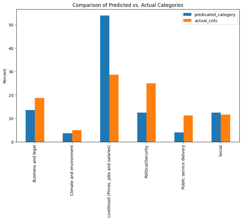
3.3.1 Compare Distributions#
In the training dataset, we check distribution (frequency distribution) for the variable category and compare it with frequency distribution for predicted_category- categories generated by LLM. Although we dont expect axact match, we expect these distributions to be comparable.
predicted_cnts = df_prot_pred.classification.value_counts(normalize=True)*100
actual_cnts = df_prot.category.value_counts(normalize=True)*100
all_labels = sorted(set(df_prot_pred.classification.unique()))
predicted_cnts = predicted_cnts.reindex(all_labels, fill_value=0)
actual_cnts = actual_cnts.reindex(all_labels, fill_value=0)

df_comparison = pd.DataFrame({'predicated_category': predicted_cnts,
'actual_cnts': actual_cnts})
Show code cell source
df_comparison.plot(kind='bar', figsize=(10,6))
plt.title("Comparison of Predicted vs. Actual Categories")
plt.ylabel("Percent")
plt.show()
Show code cell source
pretty_print_value_counts(df_prot_pred, "classification",
"Distribution of Predicted Categories",line_length=60 )
============================================================
            Distribution of Predicted Categories
============================================================
| Category | Count | Percent | Cum. Percent |
|---|---|---|---|
| Livelihood (Prices, jobs and salaries) | 13,459 | 53.93% | 53.93% |
| Business and legal | 3,369 | 13.50% | 67.43% |
| Social | 3,119 | 12.50% | 79.93% |
| Political/Security | 3,109 | 12.46% | 92.39% |
| Public service delivery | 984 | 3.94% | 96.33% |
| Climate and environment | 915 | 3.67% | 100.00% |
pretty_print_value_counts(df_prot, "category",
"Distribution of Actual Categories in Training Data",line_length=60 )
============================================================
     Distribution of Actual Categories in Training Data
============================================================
| Category | Count | Percent | Cum. Percent |
|---|---|---|---|
| Livelihood (Prices, jobs and salaries) | 64 | 28.57% | 28.57% |
| Political/Security | 56 | 25.00% | 53.57% |
| Business and legal | 42 | 18.75% | 72.32% |
| Social | 26 | 11.61% | 83.93% |
| Public service delivery | 25 | 11.16% | 95.09% |
| Climate and environment | 11 | 4.91% | 100.00% |
3.3.2 Similarity of notes within and across categories#
In order to have confidence about the classifications generated by the model, lets perform some sanity checks.
def calculate_cosine_similarity_matrix(df, categories):
    """
    Calculate a cosine similarity matrix for all categories by comparing embeddings within and across categories.

    Parameters:
    - df: DataFrame containing the 'notes' embeddings and 'predicted_category'.
    - categories: List of unique categories to compare.

    Returns:
    - similarity_matrix (pd.DataFrame): A DataFrame representing the cosine similarity matrix.
    """
    # Initialize an empty matrix for similarity scores
    similarity_matrix = np.zeros((len(categories), len(categories)))

    # Calculate cosine similarities within and across categories
    for i, category1 in enumerate(categories):
        # Filter embeddings for category1
        embeddings_category1 = np.vstack(df[df['predicted_category'] == category1]['embedding'].values)

        for j, category2 in enumerate(categories):
            # Filter embeddings for category2
            embeddings_category2 = np.vstack(df[df['predicted_category'] == category2]['embedding'].values)

            # Calculate cosine similarities between embeddings in category1 and category2
            similarity_scores = cosine_similarity(embeddings_category1, embeddings_category2).flatten()
            avg_similarity = np.mean(similarity_scores) if len(similarity_scores) > 0 else 0
            similarity_matrix[i, j] = avg_similarity

    # Convert the matrix to a DataFrame for readability
    similarity_df = pd.DataFrame(similarity_matrix, index=categories, columns=categories)
    return similarity_df
def calculate_distance_matrix(df, categories, distance_metric="euclidean"):
    """
    Calculate a distance matrix for all categories by comparing embeddings within and across categories.

    Parameters:
    - df: DataFrame containing the 'notes' embeddings and 'predicted_category'.
    - categories: List of unique categories to compare.
    - distance_metric: Type of distance to compute (e.g., 'euclidean', 'manhattan').

    Returns:
    - distance_matrix (pd.DataFrame): A DataFrame representing the distance matrix.
    """
    # Initialize an empty matrix for distance scores
    distance_matrix = np.zeros((len(categories), len(categories)))

    # Calculate distances within and across categories
    for i, category1 in enumerate(categories):
        # Filter embeddings for category1
        embeddings_category1 = np.vstack(df[df['predicted_category'] == category1]['embedding'].values)

        for j, category2 in enumerate(categories):
            # Filter embeddings for category2
            embeddings_category2 = np.vstack(df[df['predicted_category'] == category2]['embedding'].values)

            # Calculate pairwise distances between embeddings in category1 and category2
            distance_scores = cdist(embeddings_category1, embeddings_category2, metric=distance_metric).flatten()
            avg_distance = np.mean(distance_scores) if len(distance_scores) > 0 else 0
            distance_matrix[i, j] = avg_distance

    # Convert the matrix to a DataFrame for readability
    distance_df = pd.DataFrame(distance_matrix, index=categories, columns=categories)
    return distance_df
# Load dataset
df_classified_protests = pd.read_csv(DIR_DATA.joinpath("protests-labeled-all-gpt.csv"))
categories = list(df_classified_protests.classification.unique())
df_classified_protests.rename(columns={"classification":"predicted_category"}, inplace=True)
# =========================================
# LOAD AND CREATE EMBEDDINGS FOR DATAFRAME
# =========================================
# Initialize OpenAI embeddings
embedding_model = OpenAIEmbeddings(model="text-embedding-ada-002",
openai_api_type=OPENAI_API_KEY)

# Embed each note and store the embeddings in the DataFrame
df_classified_protests['embedding'] = embedding_model.embed_documents(df_classified_protests['notes'].tolist())
# =========================================
# SKLEARN COSINE SIMILARITY
# =========================================
cosine_similarity_matrix = calculate_cosine_similarity_matrix(df_classified_protests, categories)

print("="*60)
print(" Cosine Similarity Matrix (Within and Across Categories)")
print("="*60)
display(cosine_similarity_matrix)
print("-"*60)
============================================================
 Cosine Similarity Matrix (Within and Across Categories)
============================================================
| Political/Security | Livelihood (Prices, jobs and salaries) | Climate and environment | Business and legal | Social | Public service delivery | |
|---|---|---|---|---|---|---|
| Political/Security | 0.859897 | 0.824101 | 0.832180 | 0.827453 | 0.842172 | 0.831968 |
| Livelihood (Prices, jobs and salaries) | 0.824101 | 0.862665 | 0.835149 | 0.847127 | 0.836176 | 0.838875 |
| Climate and environment | 0.832180 | 0.835149 | 0.871537 | 0.835849 | 0.833948 | 0.853963 |
| Business and legal | 0.827453 | 0.847127 | 0.835849 | 0.854858 | 0.835603 | 0.838907 |
| Social | 0.842172 | 0.836176 | 0.833948 | 0.835603 | 0.856032 | 0.837756 |
| Public service delivery | 0.831968 | 0.838875 | 0.853963 | 0.838907 | 0.837756 | 0.855566 |
------------------------------------------------------------
# =========================================
# SKLEARN COSINE SIMILARITY
# =========================================
euclidean_similarity_matrix = calculate_distance_matrix(df_classified_protests, categories)

print("="*60)
print(" Euclidean Distance Similarity Matrix (Within and Across Categories)")
print("="*60)
display(euclidean_similarity_matrix)
print("-"*60)
============================================================
 Euclidean Distance Similarity Matrix (Within and Across Categories)
============================================================
| Political/Security | Livelihood (Prices, jobs and salaries) | Climate and environment | Business and legal | Social | Public service delivery | |
|---|---|---|---|---|---|---|
| Political/Security | 0.524813 | 0.592096 | 0.578313 | 0.586535 | 0.560115 | 0.578551 |
| Livelihood (Prices, jobs and salaries) | 0.592096 | 0.520636 | 0.573156 | 0.550857 | 0.570876 | 0.566408 |
| Climate and environment | 0.578313 | 0.573156 | 0.502413 | 0.572053 | 0.575235 | 0.538168 |
| Business and legal | 0.586535 | 0.550857 | 0.572053 | 0.534887 | 0.572438 | 0.566481 |
| Social | 0.560115 | 0.570876 | 0.575235 | 0.572438 | 0.532147 | 0.568317 |
| Public service delivery | 0.578551 | 0.566408 | 0.538168 | 0.566481 | 0.568317 | 0.534158 |
------------------------------------------------------------
4. Limitations and Challenges#
There are two main limitations organized in two categories as below:
Compute resource and processing time#
Although compute resources can be accessed with budget availability, LLMs generally take long to run due to the large number of parameters. In order to experiment fast, get results faster and be cost effective, sometimes you sacfrice a little bit of perfomance gains.
Classification results are not 100% accurate#
In most cases, acheiving 90% classification accuracy is good enough.Ultimately, what number counts as accurate enough varies depending on use case. In this case, we still have to live with the fact that potentially 5-10% of the classifications are wrong and there is no way to know which one. Howeever, again the sanity checks we conducted do provide a recourse to increase confidence in the results of the LLM.
5. Potential Next Steps#
Further sanity checks#
In a separate notebooks, more analysis will be done particulary focusing on time to check and demonstrate that what we got from the LLM is reasonable and matches what was happening on ground.
Further tuning of the model#
As mentioned above, the experimentation in this work was limited by available resources. Its possible to squeeze out more perfomance by utilizing a more performant OpenAI model (e.g., gpt-4o). Secondly, more experiments could be done to check to see if increasing number of examples further would improve results or whether selecting examples in a smarter way (e.g., semantic selection) which would select examples based on similary to the target note in question would yield better results. Finally, we also could try several prompting strategies to see if that also gives better perfomance.